CRWV Vs. NVDA: The "Shovel" vs. The "Mine"Why CoreWeave Offers the Higher Beta Upside IMHO!
Everyone knows NASDAQ:NVDA is the undisputed king of the AI revolution. They sell the shovels (GPUs) for the AI gold rush. But when a company reaches a multi-trillion-dollar market cap, the days of explosive, multi-bagger upside become mathematically constrained.
If you are looking for the next phase of alpha in the AI infrastructure supercycle, you have to look at the companies building the physical mines where those GPUs operate. Enter NASDAQ:CRWV (CoreWeave).
Looking at the 4-hour chart , we are seeing aggressive accumulation pushing the price back toward the $100 psychological level after shaking out weak hands in the mid-$80s. But the real story is in the fundamentals. Here is why CRWV presents a structurally higher upside potential than NVDA moving forward, along with the critical risks you must manage.
The Fundamental Symbiosis: How Both Benefit
Nvidia and CoreWeave are entirely symbiotic. AI compute demand is growing exponentially, and hyperscalers (like AWS and Azure) are struggling to keep up.
CoreWeave operates as an AI-specialized "neocloud," building massive, high-density data centers optimized specifically to run Nvidia's hardware. Nvidia benefits by selling billions in chips, and CoreWeave benefits by renting out that fully integrated compute capacity to AI labs and enterprises at a premium.
The Case for CRWV's Outsized Upside
Nvidia is essentially maxed out on valuation multiples; its growth is now a known quantity. CoreWeave, on the other hand, is uniquely positioned to capture the aggressive, physical build-out phase with far more runway:
The Nvidia Backstop: Nvidia doesn't just sell to CoreWeave; they are deeply invested. In January 2026, Nvidia directly invested another $2 billion into CRWV stock. More importantly, they established a $6.3 billion capacity agreement where Nvidia agreed to act as a backstop, promising to buy unsold compute capacity if other customers do not utilize it. Nvidia has essentially de-risked CoreWeave's expansion.
The Massive Backlog: CoreWeave’s Q2 2026 numbers were staggering. Revenue grew 112.5% year-over-year to $2.58 billion. But the true upside lies in their backlog, which currently sits at roughly $104 billion in contractually committed future revenue.
Analyst Upgrades: Wall Street is waking up to this pricing power, with major firms like Truist recently hiking their price targets to $165.
The Red Flag: The Cash Burn Monster
As a trader, I cannot ignore the elephant in the room: CoreWeave's balance sheet is stretched to the absolute limit.
This is a capital-intensive, "build-first, profit-later" model. In Q2, despite the massive revenue, CRWV posted a net loss of $626 million and suffered negative free cash flow of roughly -$5.74 billion. They are relying on aggressive debt financing (floating rate loans and massive credit facilities) to fund these data centers.
The Stabilization Thesis: This massive cash burn is a feature, not a bug, of early-stage infrastructure project financing. As their massive multi-gigawatt pipeline of data centers actively goes live over the next 12 to 18 months, capital expenditures will peak and naturally taper off. Once the infrastructure is built and the $104 billion backlog begins converting into realized operational cash flow, those margins will stabilize, and the massive debt load will become serviceable.
What is your take on this two giants?
I hear you!  Long
Long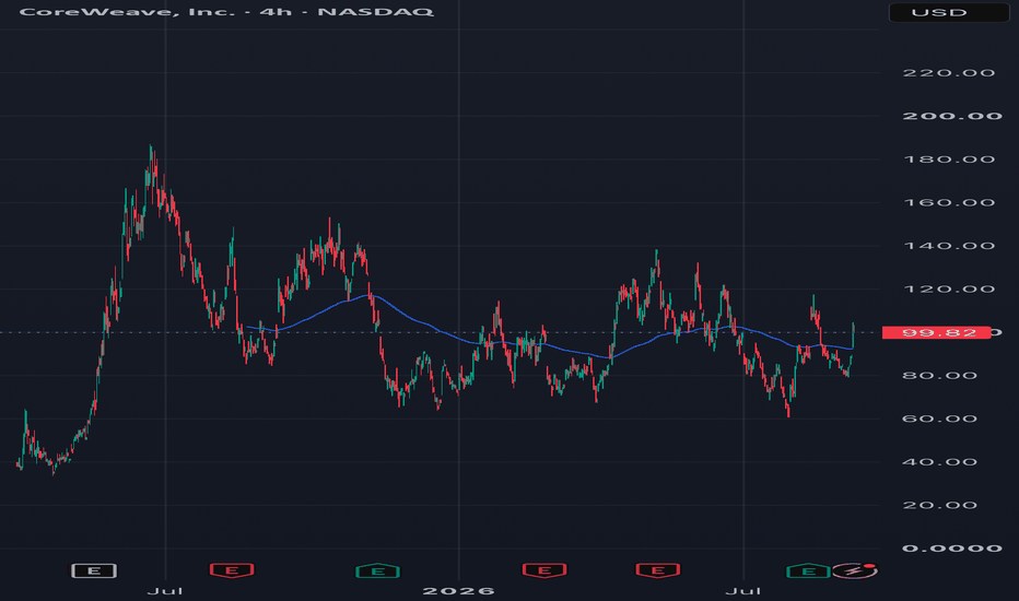
MU – Breakout Above 1000 C1, 1050 Call Wall NextMU has broken above 1000 , which serves as both the start of the call cluster and the dominant call wall in the cumulative October 16 profile. With spot near 1017.56 , price has entered positive gamma extension after consolidating above its rising 50-day moving average.
The role of 1000 has now changed from resistance to the first breakout-support test. Holding above it keeps gamma-squeeze potential open toward 1050 C2 , followed by 1100 C3 .
🔶 Regime Context 🔶
MU remains well above the 942.5 HVL , keeping the broader structure in positive GEX. GEX History shows the tracked horizons broadly aligned in positive gamma, with several shifting into extension at the right edge. The current daily breakout confirms the initial shift, but continued acceptance above 1000 is still required.
🔶 Options Structure Context 🔶
👉 1000 – C1 breakout support
Confluence at 1000:
C1 — highest call NETGEX
Ab1 — largest absolute gamma
D+ — strongest positive delta exposure
nCOI / COI — strongest net and gross call open interest
nPV / PV — strongest cumulative put volume
This makes 1000 a major two-sided reaction zone rather than only a round-number breakout.
The nearest secondary GEX peak sits at 1020 . The strongest individual call flow inside the selected horizon also appeared there for the September 9 expiration, with 21,882 contracts. Above that immediate test, 1050 C2 is the next primary call wall.
At 1100 , C3 overlaps with the strongest cumulative call and net call volume, making it the larger extension reference if momentum continues beyond 1050.
🔶 Downside Structure 🔶
👉 1000 – C1 / breakout support
👉 942.5 – HVL / regime pivot
👉 920 – P1 / strongest put wall
A move back below 1000 would return MU to the transition zone. The more consequential failure would be below 942.5 HVL , where the current positive regime would weaken. The 920 P1 also sits near the rising 50-day moving average, creating a broader support area. Below 920, the next put references are 900 P3 and 850 P2 .
🔶 Options Sentiment 🔶
CALL$ at 79.5% means calls at an equivalent distance from spot are priced 79.5% higher than corresponding puts. This is elevated call-pricing skew, not a directional guarantee.
The Options Oscillator histogram is turning sharply higher at the right edge, showing that call skew is building.
IVRank 38.5
IVx 74.2 (38 DTE) | IVx 5dCh +10.2%
CALL$ 79.5% (38 DTE) — call-pricing skew
Implied move ±2.67% (±27.2)
🔶 Key Structure to Watch 🔶
1000 — C1 breakout support and primary confluence
1020 — immediate secondary GEX and front-expiry call-flow test
1050 — C2, next primary call wall
942.5–920 — HVL-to-P1 downside structure
For now, MU remains in positive extension above 1000, but elevated call skew and rising IV increase the importance of genuine acceptance.
The key question is whether MU can hold 1000 , absorb the activity around 1020 , and continue toward 1050 , or whether the breakout returns to the transition zone. Micron Has Been SqueezingMicron Technology has consolidated for two months, and some traders may see potential for the longer-term uptrend to continue.
The first pattern on today’s chart is the narrowing range that began in late July. Bollinger Bandwidth has shrunk to the tightest level since late March. That compression may create potential for movement to resume.
Second, the memory-chip giant ended last week at its highest weekly close since late June. Prices also pushed above the 50-day simple moving average. Both signals may reflect intermediate-term bullishness.
Next, the 8-day exponential moving average (EMA) crossed above the 21-day EMA. MACD is also rising. Those signals may reflect short-term bullishness.
Finally, MU is a highly active underlier in the options market. (Its average daily volume of 921,000 contracts ranks fourth in the S&P 500, according to TradeStation data.) That could help traders take positions with calls and puts.
TradeStation has, for decades, advanced the trading industry, providing access to stocks, options and futures. If you're born to trade, we could be for you. Learn more here about TradingView’s Broker of the Year!
Past performance, whether actual or indicated by historical tests of strategies, is no guarantee of future performance or success. There is a possibility that you may sustain a loss equal to or greater than your entire investment regardless of which asset class you trade (equities, options or futures); therefore, you should not invest or risk money that you cannot afford to lose. Online trading is not suitable for all investors. View the document titled Characteristics and Risks of Standardized Options at www.TradeStation.com . Before trading any asset class, customers must read the relevant risk disclosure statements on www.TradeStation.com . System access and trade placement and execution may be delayed or fail due to market volatility and volume, quote delays, system and software errors, Internet traffic, outages and other factors.
Securities and futures trading is offered to self-directed customers by TradeStation Securities, Inc., a broker-dealer registered with the Securities and Exchange Commission and a futures commission merchant licensed with the Commodity Futures Trading Commission). TradeStation Securities is a member of the Financial Industry Regulatory Authority, the National Futures Association, and a number of exchanges.
Options trading is not suitable for all investors. Your TradeStation Securities’ account application to trade options will be considered and approved or disapproved based on all relevant factors, including your trading experience. See www.TradeStation.com . Visit www.TradeStation.com for full details on the costs and fees associated with options.
Margin trading involves risks, and it is important that you fully understand those risks before trading on margin. The Margin Disclosure Statement outlines many of those risks, including that you can lose more funds than you deposit in your margin account; your brokerage firm can force the sale of securities in your account; your brokerage firm can sell your securities without contacting you; and you are not entitled to an extension of time on a margin call. Review the Margin Disclosure Statement at www.TradeStation.com .
TradeStation Securities, Inc. and TradeStation Technologies, Inc. are each wholly owned subsidiaries of TradeStation Group, Inc., both operating, and providing products and services, under the TradeStation brand and trademark. When applying for, or purchasing, accounts, subscriptions, products and services, it is important that you know which company you will be dealing with. Visit www.TradeStation.com for further important information explaining what this means. Germany 40 – Preparing for ECB Rate Decision VolatilityJust under 2 weeks ago the Germany 40 index hit a new all-time high of 26630 on August 28th, however, since then prices have experienced a mild reversal back to the downside, with the index falling to a low of 25730 on Wednesday September 2nd before recovering slightly back to current levels around 25990 at the time of writing (0645 BST).
It seems sentiment towards some of the major German industrial corporates in the index may have been negatively impacted by the recent escalation of events in the Middle East, which is keeping energy costs elevated and may reduce margins and undermine future earnings.
Not only that, inflation in Germany, and more importantly the wider Eurozone, recently hit multi-year highs which has convinced many traders that the ECB may decide to raise interest rates again when they announce their next decision on Thursday at 1315 BST. Higher ECB interest rates tend to weigh on risk sentiment towards European stocks and vice versa.
Whether this is the case remains to be seen, but traders may also want to hear what ECB President Christine Lagarde says in the press conference (Thursday, 1345 BST) about the chances of future rate hikes moving into the end of 2026 and early 2027. Any hint at an increased potential for further ECB rate hikes to regain control of inflation could see the Germany 40 push down to create new September lows, while more dovish comments could lead to a relief rally back up towards recent highs.
Technical Update: Corrective Themes Building?:
Having posted a new all‑time high at 26630 on August 28th, the Germany 40 index has entered a corrective price phase, possibly as a reaction to what may have been over‑extended upside conditions.
However, ahead of the ECB rate decision and press conference on Thursday, traders could be attempting to establish whether this recent decline may develop into a more extended downside move, or, as has often been the case recently, price weakness proves limited before an uptrend pattern resumes.
Moving across the remainder of this week, establishing the potentially important support and resistance levels that could influence trader decision making may be useful in case Germany 40 price volatility increases into the Friday close.
Potential Resistance Levels:
While last week did see a recovery in price, it remained below what may prove to be the first potential resistance level at 26184 (the declining Bollinger mid‑average). In technical analysis, a declining mid‑average can suggest price activity is developing within a downtrend. Therefore for the Germany 40 a closing break above this mid-average may be required to indicate risks are turning back toward the upside again.
A close above 26184 could be seen as more constructive from a technical outlook and may shift the attention of traders back toward the August 28th highs at 26630 again.
A break and close above 26630 could open the way for moves toward 26962 (38.2% extension of the late‑August sell‑off).
Possible Support Levels:
While resistance at 26184 continues to cap Germany 40 prices on a closing basis, it could leave open the possibility of slowing upside momentum. If this is the case, the first support may be 25609 (38.2% retracement of the June 11th to August 28th strength).
As the chart above highlights, closing breaks below 25609 could shift focus toward the next potential support at 25294 (50% Fibonacci retracement). Closing breaks below 25294, if seen, could then open the way for declines toward 24976 (61.8% level).
The material provided here has not been prepared accordance with legal requirements designed to promote the independence of investment research and as such is considered to be a marketing communication. Whilst it is not subject to any prohibition on dealing ahead of the dissemination of investment research, we will not seek to take any advantage before providing it to our clients.
Pepperstone doesn’t represent that the material provided here is accurate, current or complete, and therefore shouldn’t be relied upon as such. The information, whether from a third party or not, isn’t to be considered as a recommendation; or an offer to buy or sell; or the solicitation of an offer to buy or sell any security, financial product or instrument; or to participate in any particular trading strategy. It does not take into account readers’ financial situation or investment objectives. We advise any readers of this content to seek their own advice. Without the approval of Pepperstone, reproduction or redistribution of this information isn’t permitted.  Long
Long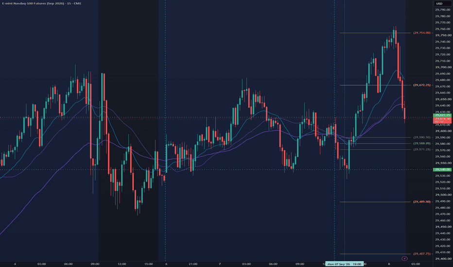
MAHARASHTRA SEAMLESS## Maharashtra Seamless Ltd. (CMP ₹689.00, NSE: MAHSCO)
**The SmartWay Research Desk | 8 September 2026**
A Mumbai‑based steel pipe## Maharashtra Seamless Ltd. (CMP ₹689.00, NSE: MAHSCOOTER)
**The SmartWay Research Desk | 8 September 2026**
A Mumbai‑based steel pipe manufacturer, incorporated in 1988. Maharashtra Seamless Ltd. is India’s largest producer of **seamless pipes, ERW pipes, and coated pipes**, catering to industries such as oil & gas, power, automotive, and infrastructure. The company is part of the DP Jindal Group and has manufacturing facilities in Maharashtra and Haryana.
**Promoter Holding (Jun 2026):** **DP Jindal Group (Jindal Family) — ~63.2% stake (no pledges)**
---
### FY22–FY26 Snapshot
- **Revenue Growth:** FY26 revenue ₹5,842 Cr vs ₹5,112 Cr in FY25 (+14.3% YoY). → **Good**
- **Net Profit:** FY26 PAT ₹812 Cr vs ₹702 Cr in FY25 (+15.7% YoY). → **Good**
- **Operating Margin:** FY26 EBITDA ₹1,412 Cr, margin 24.2% vs 23.5% last year (+70 bps). → **Good**
- **Equity Capital:** Stable, face value ₹5. → **Good**
- **Dividend Policy:** Dividend ₹6.00/share declared for FY26. → **Good**
- **Asset Building:** Investments in **capacity expansion, coated pipes, and offshore projects**. → **Good**
- **Sales:** Strong demand from **oil & gas and infra sectors**. → **Good**
- **Expense:** Raw material cost pressures (steel, alloys) remain. → **Neutral/Good**
- **EPS:** FY26 EPS ₹26.25 vs ₹22.40 last year (+17.2%). → **Good**
---
### Institutional Interest & Ownership Trends (Jun 2026)
- **Promoter Holding:** ~63.2% (no pledges)
- **FII Holding:** ~12.8%
- **DII Holding:** ~14.6%
- **Retail & Others:** ~9.4%
---
### Strategic Moves & Innovations
- Expansion in **seamless and ERW pipe capacity**.
- Focus on **oil & gas exploration and offshore projects**.
- Partnerships with **global energy companies for supply contracts**.
- Diversification into **coated pipes and specialized industrial products**.
---
### Cash Flow & Balance Sheet Strength
- Market cap ~₹11,200 Cr.
- Debt‑to‑equity ratio ~0.42 (moderate leverage).
- Book value per share ₹182.00; P/B ~3.8.
- EPS (TTM) ₹26.25; P/E ~26.2.
---
### Risk Factors
- Moderate‑high **P/E ratio ~26.2**, valuations slightly expensive.
- Dependence on **oil & gas demand cycles**.
- Exposure to **commodity price volatility (steel, alloys)**.
- Competition from Ratnamani Metals, Welspun Corp, and Jindal SAW.
---
### Investor Takeaway
Maharashtra Seamless has delivered **robust FY26 performance**, supported by demand in oil & gas, infra projects, and coated pipe expansion. With strong promoter backing (Jindal Family, 63.2% stake), dividend payouts, and leadership in seamless pipes, the company remains a **mid‑cap steel & infra play**. At CMP ₹689.00, valuations are **moderately expensive (P/E ~26.2, P/B ~3.8)**, reflecting growth expectations with manageable risks.  Long
Long
INTC – Bounce from 85 Put Wall, Watching 100 Call WallINTC is bouncing off the 85 put wall on the daily chart, with price now holding near 95.61 after reclaiming the 90 HVL. On the October 16 cumulative GEX Profile, that keeps INTC in a positive GEX regime (spot above HVL) and inside the call cluster above 93 (cTrans). The 100 call wall is still overhead — this is not yet a positive-extension story on that swing profile.
🔶 Regime Context 🔶
Price is trading above HVL at 90 , so the regime read is positive. GEX History on the daily is an all-green map, but size splits the story : the shortest two rows (0 and W1) print large green — those front expirations are in positive extension, consistent with spot already through their call walls near 95. M1, M2, and ALL stay smaller green : positive gamma, not through the 100 C1 of the October 16 cumulative map. That is not all-expiry extension confluence. The path still matters — the panel shifted out of a broad red stretch as price bounced from 85. That bounce is the momentum confirmation so far; 100 is where the next confirmation is required.
🔶 Options Structure Context 🔶
👉 100 – C1 — highest call NETGEX on the October 16 cumulative profile (42 DTE)
Call volume on the October 16 expiry itself also peaks at 100 .
👉 95 – C3 + Ab1 — largest absolute gamma, sitting right under spot
Confluence at 95 (October 16, 42 DTE, cumulative):
C3 — third call wall
Ab1 — largest absolute gamma
D+ — strongest positive delta exposure
That makes 95 a clear reaction zone, not just a round number — price is holding this cluster while stretching toward 100.
👉 110 – C2 — next call wall, and the heavier inventory/flow cluster above C1
Confluence at 110 (October 16, 42 DTE, cumulative):
C2 — second call wall
COI — highest call open interest
AbOI — highest absolute open interest
CV / nCV — strongest call volume (cumulative)
If 100 is accepted, positive extension opens toward 110, with gamma squeeze potential only if momentum holds above C1.
🔶 Downside Structure 🔶
👉 90 – HVL / P3 — regime pivot; must hold for the positive-regime read
👉 85 – P1 — strongest put wall; the bounce origin
Confluence at 85 (October 16, 42 DTE, cumulative):
P1 — strongest put wall
PV / nPV — strongest put volume
Together, this is the put-side reaction zone that launched the bounce.
👉 80 – P2 / POI / nPOI — next put cluster if 85 fails
🔶 Options Sentiment 🔶
CALL$ 66% (42 DTE) means call options at an equivalent distance from spot are priced 66% higher than the corresponding puts — this is call pricing skew .
On the Options Oscillator, the filled green histogram remains elevated on the right edge — call pricing skew is holding at a high level , not fading.
IVRank 22.5
IVx 59.2 (42 DTE)
CALL$ 66% (42 DTE) — call pricing skew
Implied move ±1.76%
🔶 Key Structure to Watch 🔶
100 — C1; the decision for swing-horizon extension
95 — C3 + Ab1; current magnet
90 — HVL; regime pivot
85 — P1; bounce support
For now, INTC is a put-wall bounce holding above HVL, with only the front History rows in extension.
The key question is whether momentum can carry price through 100 — or whether the call wall rejects and sends the test back toward 90. Long 
US 500 – Preparing For Payrolls VolatilityYesterday the US 500 index rallied 0.3%, breaking a losing streak that had extended to 3 days immediately following the comments made by Federal Reserve Chair Kevin Warsh from the Jackson Hole on Friday, that were deemed to be more hawkish than many traders had been expecting and positioning for.
Interestingly, the 3-day decline held against a potentially important technical level, (more detail in technical section below) with traders seemingly happy to buy the dip while US corporate earnings remain solid and the oil price drops back slightly from 6-week highs.
However, despite the rebound in prices from their lows around 7615, trader uncertainty remains regarding the unstable situation in the Middle East, the impact of rising inflation on Fed interest rate policy and the outcome of this Friday’s US Non-farm Payrolls release (1330 BST). All of which has combined to help keep volatility elevated moving towards the weekend.
Looking forward to Friday’s US jobs report, while the headline number is often volatile, sentiment and positioning in the US 500 may be influenced by whether the unemployment rate moves above or below its current level of 4.1% and by the relative strength of average hourly earnings. Any deviation from market expectations may impact the decision making of Fed policymakers when they meet on September 16th to decide their next rate move. This could mean the payrolls outcome may have direct implications for the short-term direction of the US 500 back up towards all-time highs at 7817 (August 13th), or perhaps down towards new lows below 7615.
Technical Update: Price Weakness Finding Support at 38.2% Fibonacci Retracement Level
Having posted a new all‑time high at 7817 (August 13th), the US 500 index has entered a period of price consolidation. This type of activity is often seen after a strong advance, acting as a natural reaction to what were perhaps over‑extended upside conditions.
The challenge for traders in this environment may be attempting to determine whether the latest price weakness is, as has been the case previously, a limited downside correction from which fresh strength can reemerge, or if it represents a more meaningful negative sentiment shift that could lead to further deeper declines. For the upcoming sessions into the Friday close it could be useful to identify potential key support and resistance levels that may play an important role in shaping the next directional themes.
Potential Support Levels:
Recent declines in the US 500 on Tuesday and Wednesday this week have been held by what may be seen as important support at 7615 (38.2% retracement of the July 29th to August 13th upside). This could represent the first key level for traders to focus on over the next 48 hours.
Closing breaks below 7615, while not a guarantee of further declines, could trigger a deeper retracement of the price strength developing from the July 29th low. Breaks of 7615 could open scope toward 7534 (50% Fibonacci retracement), and possibly then 7492, (deeper 61.8% level).
Potential Resistance Levels:
While support at 7615 (38% retracement) remains intact on a closing basis, fresh attempts to push back towards the upside could emerge. In this scenario, the focus for traders may be on potential resistance at 7708 (Bollinger mid‑average).
Closing breaks above 7708 could lead to further price strength to challenge the August 28th high at 7771 and, if this level were also to give way, back to 7817 (August 13th high).
The material provided here has not been prepared accordance with legal requirements designed to promote the independence of investment research and as such is considered to be a marketing communication. Whilst it is not subject to any prohibition on dealing ahead of the dissemination of investment research, we will not seek to take any advantage before providing it to our clients.
Pepperstone doesn’t represent that the material provided here is accurate, current or complete, and therefore shouldn’t be relied upon as such. The information, whether from a third party or not, isn’t to be considered as a recommendation; or an offer to buy or sell; or the solicitation of an offer to buy or sell any security, financial product or instrument; or to participate in any particular trading strategy. It does not take into account readers’ financial situation or investment objectives. We advise any readers of this content to seek their own advice. Without the approval of Pepperstone, reproduction or redistribution of this information isn’t permitted.
Short 
Sharpe Ratio Part 2: 5 Common Calculation Errors📊 Sharpe Ratio Part 2: 5 Common Calculation Errors
The Sharpe Ratio is one of the most widely used measures of risk-adjusted performance, but even a mathematically correct formula can produce a misleading result if the underlying data, sampling frequency, or methodology is handled incorrectly.
In Part 1, we examined how the Sharpe Ratio can be applied to stocks, portfolios, trading strategies, and rolling analysis.
🔁 The basic formula is:
Sharpe = (Rₚ − Rf) / σₚ
Where:
Rₚ = portfolio or strategy return
Rf = risk-free rate
σₚ = standard deviation of returns
Part 2 focuses on five common calculation errors that can distort Sharpe Ratio values or make otherwise valid values difficult to compare.
---
📌 5 Common Calculation Errors
1️⃣ Improper Annualization
The Sharpe Ratio is fundamentally a ratio of average excess return to return volatility. If you calculate it from daily returns, the result is a daily Sharpe Ratio. If you want to compare it with a yearly Sharpe Ratio, you must annualize both components consistently.
Sharpe_annual = Sharpe_period × √(periods per year)
Sharpe does not scale linearly with time — it scales with the square root of time.
For daily data, the common approximation is:
Sharpe_annual = Sharpe_daily × √252
For example, a daily Sharpe of 0.10 becomes approximately 0.10 × √252 ≈ 1.59.
The number 252 represents the commonly used approximation for trading days in a year.
A common mistake is to multiply the Sharpe Ratio by 252 rather than √252, or to annualize the return while leaving volatility on a different time scale. Either approach can produce a substantially distorted result.
📋 Common Annualization Multipliers
• Hourly (US Stocks) — 1,638 hours (252 days × 6.5 hrs) → √1,638 ≈ 40.47
• Hourly (Crypto, 24/7) — 8,760 hours (365 days × 24 hrs) → √8,760 ≈ 93.59
• Daily (Traditional Markets) — 252 days → √252 ≈ 15.87
• Daily (Crypto, 24/7) — 365 days → √365 ≈ 19.10
• Weekly — 52 weeks → √52 ≈ 7.21
• Monthly — 12 months → √12 ≈ 3.46
From the chart above, it is evident that once both series are annualized with their appropriate scaling factors (√252 for daily and √1,638 for hourly), the daily and hourly Sharpe curves track each other closely across the full 2021–2025 period, showing similar cycles and sign changes with broadly comparable magnitudes. Without annualization, the same two series diverge sharply in scale: the raw daily Sharpe peaks near 0.31 while the raw hourly Sharpe peaks near 0.10 around April 2024. Although both are derived from the same underlying price series, they are calculated from different return frequencies. Comparing those raw values directly could therefore suggest that daily performance is roughly three times better than hourly — a misleading conclusion driven by the different sampling frequencies and time scales rather than by a genuine difference in risk-adjusted performance.
📌 Why it matters
If a Sharpe of 1.2 from daily returns is reported and compared to a Sharpe of 1.2 from weekly returns, those numbers are not comparable. A Sharpe Ratio without knowing its calculation frequency and annualization method can be misleading.
💡 Note on Custom Session Hours: For assets traded outside standard hours (e.g., markets with 7-hour or 8-hour sessions, extended/pre-market trading, or Gold and Forex), calculate your hourly multiplier as:
Periods per year = 252 × Session Hours per Day
The annualization factor is then:
√(Periods per year)
⚠️ Annualization is only meaningful when the underlying return observations and scaling assumptions are appropriate for the asset and timeframe.
---
2️⃣ Using Cumulative Return Instead of Periodic Returns
The Sharpe Ratio should be calculated from a series of periodic returns, not from the cumulative return over the entire period.
For example, suppose an asset produces these monthly returns:
+10%, −5%, +3%, −2%
The Sharpe calculation needs the individual monthly returns because it needs to measure both:
• the average return
• the variability of those returns
If the asset instead has a cumulative return of +5% over the entire period, using that +5% as a single Sharpe input removes the information about how the return was achieved.
Two assets could both produce a 20% total return, while one achieved it smoothly and the other experienced large gains and losses. Their risk-adjusted performance can therefore be very different.
📌 Why it matters
A cumulative return tells you what happened between two points in time.
The Sharpe Ratio is intended to evaluate how efficiently returns were generated relative to the variability of the return stream.
Using cumulative performance as though it were a periodic return series destroys that distinction and can result in an invalid and misleading Sharpe calculation.
---
3️⃣ Ignoring the Statistical Assumptions
The traditional Sharpe Ratio works best under assumptions that are often unrealistic for financial markets:
• returns have reasonably stable volatility
• observations are independent
• returns are approximately normally distributed
Real market returns frequently violate one or more of these assumptions, which can make the conventional Sharpe Ratio an incomplete or potentially misleading measure of risk-adjusted performance.
Volatility is not necessarily stable.
A stock can spend months with low volatility and then enter a highly volatile regime, a phenomenon referred to as volatility clustering. A single Sharpe Ratio calculated over the entire period can hide this change.
Returns are not necessarily independent.
Serial correlation can occur in financial time series, particularly in certain strategies, assets, or timeframes. If returns are correlated, the standard volatility calculation may not adequately represent the true risk of the return stream. Lo (2002) showed that positively autocorrelated returns (common in strategies with smoothing, options overlays, or illiquid instruments) inflate the standard annualized Sharpe.
Returns are not necessarily normally distributed.
Financial returns often exhibit fat tails and skewness. Large negative observations can occur much more frequently than a normal distribution would suggest.
📌 Why it matters
A Sharpe Ratio of 1.5 does not automatically mean a strategy has "good risk-adjusted performance" under every market condition. A strategy can have an attractive Sharpe while still being exposed to large tail losses, volatility clustering, or changing market regimes.
This is one reason why Sharpe should be viewed alongside metrics such as Maximum Drawdown, Sortino Ratio, Ulcer Index, and Martin Ratio, rather than used in isolation.
Adjustments to the standard Sharpe have been made to address some of these assumptions. The autocorrelation-adjusted scaling factor (Lo, 2002) corrects for serial dependence. The Deflated Sharpe Ratio (Bailey & López de Prado) addresses issues such as non-normal returns and selection bias arising when many strategies or variations are tested. Other methodologies have also been developed to address regime-dependent volatility
---
4️⃣ Comparing Tickers Across Different Timeframes
A Sharpe Ratio calculated from daily returns and one calculated from hourly returns are based on different return series. The change in sampling frequency can affect both the measured average return and the measured volatility.
For example:
• Stock A: Sharpe = 1.20 on daily data
• Stock B: Sharpe = 1.20 on hourly data
It may be tempting to conclude that both stocks have the same risk-adjusted performance. However, the two values are based on different sampling frequencies and therefore do not necessarily describe the same return dynamics.
This is different from **annualization**. Annualization adjusts a Sharpe Ratio calculated at a particular frequency to a common time basis. It does not make Sharpe Ratios calculated from fundamentally different return series equivalent.
The distinction is particularly important on TradingView, where users routinely switch between 1-minute, 5-minute, 1-hour, 4-hour, daily, and weekly charts. Changing the timeframe changes the observations used to calculate the Sharpe Ratio, which can materially change the resulting value even when each Sharpe is correctly annualized.
📌 Why it matters
When comparing Sharpe Ratios across tickers, use the same calculation timeframe and methodology whenever possible. If different timeframes must be used, annualization can put the results on a common time scale, but it does not eliminate the differences caused by the underlying sampling frequency.
A screener or indicator that compares Sharpe Ratios calculated from different return frequencies can therefore produce misleading rankings, even when the individual Sharpe calculations are mathematically correct.
---
5️⃣ Calculating Sharpe From Trade Logs Instead of the Time Series
As covered in Part 1, the preferred approach is Equity Curve → Periodic Returns → Excess Returns → Sharpe. This error is what happens when that order is skipped.
This is particularly important when evaluating TradingView strategies. Suppose a strategy generates 20 trades. A user takes the profit/loss percentage of each completed trade and calculates:
Sharpe = Average Trade Return / STD(Trade Return)
It may look mathematically reasonable — but this is not necessarily the conventional Sharpe Ratio of the strategy's investment returns.
The problem is that individual trades are not necessarily equivalent observations in time.
Trades can have:
• different holding periods
• different amounts of capital at risk
• overlapping positions
• periods when the strategy is completely out of the market
• different levels of market exposure over time
A trade lasting two days and a trade lasting six months are both counted as one observation in a simple trade-log calculation, even though they represent very different amounts of time exposure.
For conventional strategy performance analysis, Sharpe is generally calculated from a time series of portfolio or strategy returns, such as periodic returns derived from the equity curve.
For example:
rₜ = (Equityₜ / Equityₜ₋₁) − 1
The resulting periodic return series can then be used to calculate the mean return and standard deviation consistently through time.
📌 Why it matters
The Sharpe Ratio is intended to describe the quality of a return stream through time, not simply the average quality of individual trades.
A strategy can have a high average trade return but a mediocre Sharpe if it spends long periods idle or experiences substantial volatility in its equity curve.
Likewise, a trade-based Sharpe can be misleading when trade durations, capital exposure, and time between trades are ignored.
A trade-level statistic can still be useful, but it should be clearly identified as a *trade-level Sharpe* rather than presented as the conventional time-series Sharpe Ratio.
---
🏁 Final Takeaway
A Sharpe Ratio is only as meaningful as the return series and methodology behind it.
A seemingly precise Sharpe value can be misleading if the underlying returns are sampled or annualized incorrectly, if the statistical characteristics of those returns are ignored, or if values calculated using different methodologies are compared directly.
For trading strategies, the calculation should generally reflect the strategy's return stream through time rather than simply the outcomes of individual trades.
📌 The formula may be simple. Producing a meaningful Sharpe Ratio requires careful treatment of the data behind it.
---
📝 Note
Sharpe Ratio applications and methodologies are extensive. Interested users should explore additional approaches for evaluating risk-adjusted performance using the Sharpe Ratio.
Sharpe Ratio — Educational TrendAdvantage Reference
 Education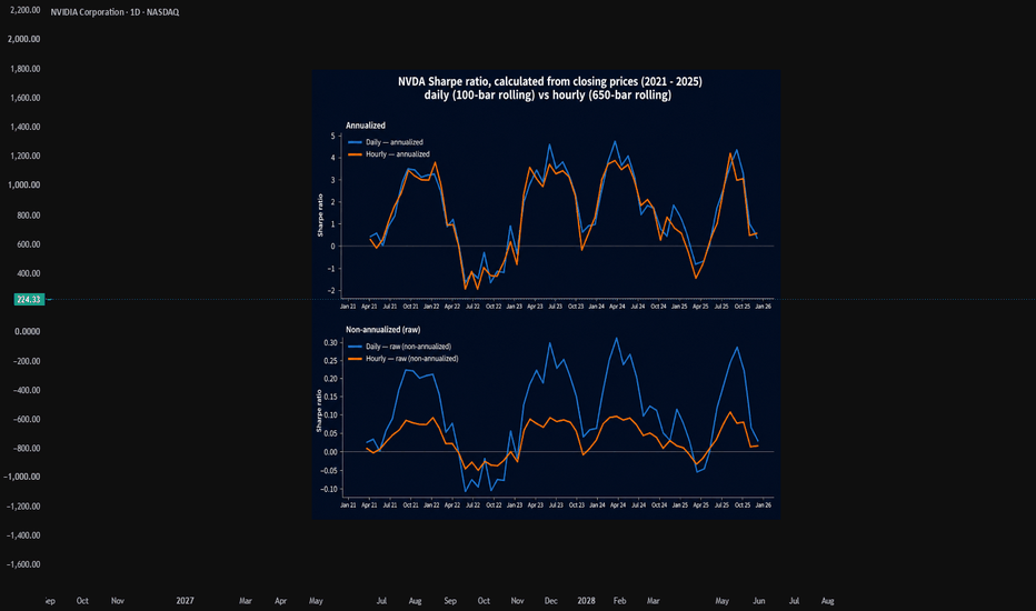
Buy opportunity on EUR/AUDThere aren't many factors for this trade; hence I entered with half the risk. Nonetheless, these are still quite powerful.
Firstly, while the lower time frames (using the 200 MA) show a downtrend, the trend is still up on the monthly time frame.
Going outside the charts, the latest Commitment of Traders report shows that leveraged funds have added 19,357 long contracts and are at a negative percentile extreme. These are two hints of potential bullishness.
Finally, using my own analysis of economic releases over several weeks, the euro has been the strongest in producing positive results, while the Aussie is sixth-highest.
My entry point is at 1.61750, the first standard deviation level when considering today's realized volatility. Meanwhile, the stop is at 1.61512. ORCL GEX – 140 Put Wall Holds, 160 Call Wall in FocusORCL continues to defend 140 after several tests, making this the central level in the current structure.
In the October 16 cumulative profile, 140 is more than the strongest put wall. It also carries the largest absolute gamma and the dominant put-volume strike, creating a clear reaction zone.
🔶 Regime Context 🔶
Spot at 144.98 is above the 143 HVL, keeping ORCL on the positive side of the GEX regime pivot. However, price remains below cTrans at 149, so it is still inside the transition zone rather than the call cluster.
A reclaim of 149–150 would be the first structural improvement.
🔶 Support Confluence 🔶
👉 140 – P1 / Ab1 / PV
Confluence at 140 — October 16 cumulative profile, 44 DTE:
P1 — strongest put wall
Ab1 — largest absolute gamma
PV — dominant put-volume strike
Repeated defenses of this level show why 140 remains the structural floor. A clear break below it would open the negative extension zone, with 125 and 120 as the next lower references.
🔶 Upside Structure 🔶
👉 149 – cTrans , start of the call cluster
👉 150 – C2 , nearest call wall
👉 155 – C3 , secondary call wall
👉 160 – C1 / D+ / nCV / CV
Confluence at 160 — October 16 cumulative profile, 44 DTE:
C1 — highest call NETGEX
D+ — strongest positive delta exposure
nCV / CV — dominant call-volume concentration
This makes 160 the primary upside reaction zone. Acceptance above it would move ORCL into the positive extension zone and introduce gamma squeeze potential.
🔶 Options Sentiment 🔶
CALL$ 56.2% means calls at an equivalent distance from spot are priced 56.2% higher than the corresponding puts. This is elevated call pricing skew, but not a directional guarantee.
The Options Oscillator’s green histogram is declining from a recent peak, showing that call pricing skew is fading despite remaining positive.
IVRank 55.9
IVx 67.8 (44 DTE) | IVx 5dCh −2.1%
CALL$ 56.2% (44 DTE) — call pricing skew
Implied move ±3.42% (±4.92)
🔶 Key Structure to Watch 🔶
143 — HVL and regime pivot
149–150 — transition exit and first call wall
160 — major call-side confluence
140 — principal downside reaction zone
For now, ORCL is holding above its key put-wall confluence but has not yet entered the call cluster.
The key question is whether 140 can continue to hold while price reclaims 149–150—or whether another rejection sends ORCL back toward the structural floor. SoFi Might Be SlippingSoFi Technologies has limped most of the year despite the broader S&P 500 hitting new highs. Does that lack of relative strength reveal underlying weakness?
The first pattern on today’s chart is the drop in the first quarter. Prices made some feeble attempts at recovery, but each time made lower highs. That could reflect a lack of buying interest.
Second, the 50-day simple moving average (SMA) had a “death cross” under the 200-day SMA in March. That could also suggest that a longer-term downtrend has begun.
Third, prices returned under the 50-day SMA this week. That may signal intermediate-term weakness.
Fourth, the 8-day exponential moving average (EMA) crossed under the 21-day EMA. MACD is also falling. Those signals may be consistent with short-term bearishness.
Next, the financial stock’s recent period of sideways movement has caused Bollinger Bandwidth to narrow. Such price compression could lay the groundwork for expansion.
Finally, SOFI is an active underlier in the options market. (If it were a member of the S&P 500, its average daily volume of 340,000 contracts would rank 12th, according to TradeStation data.) That could help traders take positions with calls and puts.
TradeStation has, for decades, advanced the trading industry, providing access to stocks, options and futures. If you're born to trade, we could be for you. Learn more here about TradingView’s Broker of the Year!
Past performance, whether actual or indicated by historical tests of strategies, is no guarantee of future performance or success. There is a possibility that you may sustain a loss equal to or greater than your entire investment regardless of which asset class you trade (equities, options or futures); therefore, you should not invest or risk money that you cannot afford to lose. Online trading is not suitable for all investors. View the document titled Characteristics and Risks of Standardized Options at www.TradeStation.com . Before trading any asset class, customers must read the relevant risk disclosure statements on www.TradeStation.com . System access and trade placement and execution may be delayed or fail due to market volatility and volume, quote delays, system and software errors, Internet traffic, outages and other factors.
Securities and futures trading is offered to self-directed customers by TradeStation Securities, Inc., a broker-dealer registered with the Securities and Exchange Commission and a futures commission merchant licensed with the Commodity Futures Trading Commission). TradeStation Securities is a member of the Financial Industry Regulatory Authority, the National Futures Association, and a number of exchanges.
Options trading is not suitable for all investors. Your TradeStation Securities’ account application to trade options will be considered and approved or disapproved based on all relevant factors, including your trading experience. See www.TradeStation.com . Visit www.TradeStation.com for full details on the costs and fees associated with options.
Margin trading involves risks, and it is important that you fully understand those risks before trading on margin. The Margin Disclosure Statement outlines many of those risks, including that you can lose more funds than you deposit in your margin account; your brokerage firm can force the sale of securities in your account; your brokerage firm can sell your securities without contacting you; and you are not entitled to an extension of time on a margin call. Review the Margin Disclosure Statement at www.TradeStation.com .
TradeStation Securities, Inc. and TradeStation Technologies, Inc. are each wholly owned subsidiaries of TradeStation Group, Inc., both operating, and providing products and services, under the TradeStation brand and trademark. When applying for, or purchasing, accounts, subscriptions, products and services, it is important that you know which company you will be dealing with. Visit www.TradeStation.com for further important information explaining what this means. Bitcoin – Is the Short Term Top in Place?The cryptocurrency market exploded back into life at the back end of August, taking Bitcoin quickly out of a drab summer trading range between 57699 (July 1st low) and 67258 (July 22nd high), adding 24% to its price in just 2 weeks in a move which achieved a 3 month high at 81554 before running into a wall of profit taking ahead of some important technical levels, more on this in the update below.
Now, with the Bitcoin price back trading around 77500 again at the time of writing (0645 BST), as general risk sentiment cools at the start of September due to surging global yields, an escalation of the Iran conflict, alongside worries about inflation and the potential for a Fed rate hike in September, the question Bitcoin traders could be asking themselves is, where next for the world’s biggest cryptocurrency?
Looking forward, much could depend on the assessment of the short-term technical outlook and how the price of Bitcoin performs when potentially important support or resistance levels are tested or even broken.
Technical Update: Why 82827-83156 May Be a Key Resistance Focus:
In true Bitcoin style, the last two weeks of August caught many traders off‑guard, as a sharp 30.5% rally developed from the August 14th low at 62458 up to the August 28th high of 81554. The sheer speed of this unwinding of bearish positioning left many traders racing to catch up.
However, as the weekly chart above shows, the latest price strength has approached what may prove to be a key resistance zone between 82827-83156 (the May 2026 recovery high and the 38.2% retracement of the October 2025 to July 2026 decline).
Potential Resistance Focus:
In technical analysis, a last recovery high and failure point of a previous downtrend may often be monitored closely by traders as a key resistance level. For Bitcoin, the May 2026 high stands at 82827. The fact this point is also close to 83156 (38% retracement) adds to the potential importance of the 82827-83156 zone as a resistance focus. If Bitcoin is to attempt further upside, it could well be closes above 82827-83156 that are required to suggest it.
As the above weekly chart shows, closing breaks above 82827-83156, could shift focus to 91,068 (50% Fibonacci retracement). Closes above 91,068, might open the way for moves toward 98,979 (61.8% Fibonacci level).
Potential Support Focus:
While the 82827-83156 resistance zone continues to cap prices a fresh sell‑off is still possible. In this scenario the focus for traders may shift to 76329 which is the September 1st low as the first key support level. Closes below 76329, while not guaranteeing further weakness, could lead to further declines.
As the daily chart above shows, closes below 76329 could open potential for moves toward the next support at 74340 (38.2% retracement) and, if this level also gives way, on toward 72087 (50% retracement).
The material provided here has not been prepared accordance with legal requirements designed to promote the independence of investment research and as such is considered to be a marketing communication. Whilst it is not subject to any prohibition on dealing ahead of the dissemination of investment research, we will not seek to take any advantage before providing it to our clients.
Pepperstone doesn’t represent that the material provided here is accurate, current or complete, and therefore shouldn’t be relied upon as such. The information, whether from a third party or not, isn’t to be considered as a recommendation; or an offer to buy or sell; or the solicitation of an offer to buy or sell any security, financial product or instrument; or to participate in any particular trading strategy. It does not take into account readers’ financial situation or investment objectives. We advise any readers of this content to seek their own advice. Without the approval of Pepperstone, reproduction or redistribution of this information isn’t permitted. Short 
NTSK a special Crawler working its way slow but steadyNetskope (NTSK) has established a definitive technical floor in the high $12 to low $13 range, a level perfectly aligned with a recent wave of heavy insider accumulation. As illustrated in the provided image_2.png, price action is curling out of this demand zone, underpinned by a massive fundamental tailwind in enterprise artificial intelligence and cybersecurity.
The Technical Picture & Insider Alignment
As seen in image, NTSK carved out a rigid support shelf right around the $12.83 mark. Selling pressure has dried up entirely at this level, and current price action near $14.04 suggests a structural reversal is underway. This technical floor is being actively defended by institutional and insider capital:
William J.G. Griffith, a company director, recently acquired over 300,000 shares for roughly $3.76 million. His purchases were executed at weighted average prices between $12.25 and $12.42, perfectly matching the technical support zone shown on the chart.
ICONIQ Strategic Partners, an entity connected to 10% owner Divesh Makan, acquired an additional $3.77 million in stock at those exact same price levels.
Netskope's Cloud Security Model
Netskope operates natively in the Secure Access Service Edge (SASE) and Security Service Edge (SSE) sectors. As corporations abandon traditional centralized data centers for hybrid work environments, legacy perimeter defenses like standard VPNs and firewalls are becoming obsolete. The flagship "Netskope One" platform unifies networking and security into a single cloud-delivered architecture, protecting users, applications, and data regardless of their physical location.
The Enterprise AI Catalyst
The explosive adoption of generative AI across corporate environments serves as Netskope's most significant growth multiplier.
Corporations are increasingly terrified of employees accidentally leaking proprietary data into public AI models.
Netskope leverages patented AI and machine learning techniques within its Zero Trust Engine to continuously monitor and adapt security protocols based on user context and interaction.
Their advanced Data Loss Prevention (DLP) systems are specifically engineered to safeguard data across native and embedded generative AI applications. This allows IT departments to securely enable AI usage without the risk of data exfiltration, positioning Netskope as a mandatory infrastructure layer for the AI boom.
Holding the $12.83 structural support shown in image is the key to validating this bottoming thesis. A sustained break above local resistance around the mid-$15s will confirm the macro uptrend, heavily supported by smart money inflows and AI cybersecurity tailwinds.
Disclaimer: This analysis is for educational purposes only and does not constitute financial advice.  Long
Long