Market Rotor - Rotation Artifact Null Test [FibonacciFlux]
Market Rotor is the first of a series of published experiments: take a correction that is widely assumed to work, implement it honestly, and find out what it actually does. This one tests the standard artifact correction for cross-sectional rotation - the claim that you can estimate each asset's own autocorrelation, subtract the rotation that autocorrelation implies, and treat whatever is left as genuine lead-lag.
Implemented and measured, it does not do that. The script is published so the test can be repeated and the result attacked.
🔶 USAGE
🔹 What this is for
Before you build on, or believe, a rotation or lead-lag indicator, load your basket here. If an artifact component is identified, an artifact component is present in the rotation this basket produces at this window - which is reason to check whether the indicator you were about to trust is reading the same thing. If nothing is resolved, you have learned that this particular correction cannot tell you either way - which is worth knowing, because the correction is usually assumed to work rather than checked.
🔹 Reading the shading
The background has two states and neither of them is an all-clear:

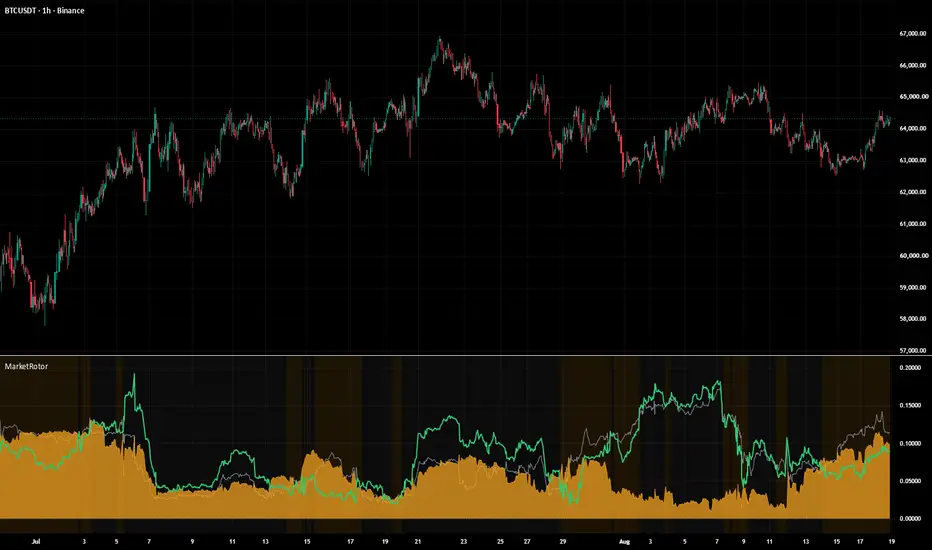
Two months of BINANCE:BTCUSDT 1H at the defaults. The two states alternate throughout - there is no long stretch where the correction cleanly resolves anything.
There is deliberately no green state anywhere in this script. A reassuring colour would be the most misleading thing it could draw, because the test is structurally incapable of certifying that an observed rotation is real.
🔹 Reading the plots
Three Frobenius norms share the pane. Grey is the observed rotation, the amber filled area is the artifact estimate, green is the residual. These are matrix norms, not components: they do not sum, and the residual can and often does exceed the observed norm. When it does, subtracting the artifact estimate has added variance rather than removed it - see the noise floor below.
The Data Window carries the quantities that actually matter: R-squared, the residual share, the direction agreement cos(Ω, Ω_art), the mean off-diagonal of G0, the four estimated AR(1) coefficients, the effective sample count, and the legacy statistic from the first version of this script, kept only for comparison.
🔹 Choosing the symbol set
The artifact term is proportional to contemporaneous co-movement. If your four assets barely co-move, or their bars do not align - mixing a stock with 24/7 crypto is the common case - the artifact estimate collapses toward zero for reasons that have nothing to do with lead-lag, and the test silently becomes vacuous. Watch the mean off-diagonal of G0 in the Data Window: if it is small, the reading means nothing.

The same script on NASDAQ:AAPL daily with the three Binance defaults left in place - the first thing most readers will try. Nothing warns you. On the bar shown, the mean off-diagonal of G0 falls from 0.87 to 0.34, the artifact estimate collapses with it to 0.016 against an observed norm of 0.081, cos(Ω, Ω_art) reads -0.85, and the residual ends up larger than the observed rotation it came from. Note what the old v1 statistic does here: 0.20, which under that version's bands was its most reassuring possible reading. The tool's least trustworthy configuration was the one it praised.
Requests use gaps_on, so a symbol with a missing bar yields na and that bar is skipped rather than having a stale return carried into the estimate.
🔹 Warm-up and repainting
Nothing plots until the window is full and W + z-score-length bars have elapsed: 500 bars at the defaults, roughly three weeks of 1H data, but around two years on a daily chart. If the pane is empty, that is why. The accumulator only advances on confirmed bars, so historical values do not repaint.
🔶 DETAILS
🔹 The identity being tested
Let each asset follow its own AR(1) with coefficient phi_i, and let the true cross-asset lead/lag be identically zero:
Pine Script®
Exact in population. The proposal it suggests - estimate phi from each asset's own autocorrelation, form the implied artifact, subtract it, call the remainder genuine lead-lag - is what this script implements so that it can be tested rather than assumed.
🔹 Where the numbers come from
The core was reimplemented outside Pine and agrees with this script to five decimal places on the same bar; every figure below comes from that reimplementation. Figures labelled synthetic are generated with a seeded generator and known ground truth, so they reproduce exactly. Real-data figures name the symbol, timeframe and window they were taken on, and the two single-bar readings are marked as such.
🔹 Result 1: the correction is not identified
phi_i estimated from asset i's own autocorrelation cannot distinguish "asset i is autocorrelated" from "asset i is led by asset j", because the second necessarily produces the first. On synthetic data where a genuine lead-lag is injected, the artifact model fits better, not worse: R-squared rises to +0.40 and cos(Ω, Ω_art) to +0.74 at W=250. The correction absorbs precisely the thing it is meant to leave behind.
🔹 Result 2: the subtraction is noise-dominated
Ω is estimated from the off-diagonal of G1; the artifact term from the diagonal of G1 plus G0. Under the null these estimate the same population quantity. If their errors are of comparable size and not strongly correlated, Var(Ω_res) = Var(Ω) + Var(Ω_art) and the residual share tends to sqrt(2) = 1.414 when noise dominates. Both of those are assumptions rather than results - the two estimators are built from the same return pairs over the same window, and the null identity ties them together - so read the measured spread as the test of them, not as a confirmation of the algebra. On synthetic all-artifact data it lands between 1.10 and 1.88, straddling that value, and the finding that survives either way is that the residual is larger than the quantity it was subtracted from. On BINANCE:BTCUSDT 1H with the default basket at W=250, the median R-squared is about -0.7 - near the noise floor of -1.
🔹 What the first version of this script got wrong
Version 1 shaded on ‖Ω_art‖ / ‖Ω‖. That statistic compares magnitudes only and is not a fraction-explained, because the artifact and residual matrices are not orthogonal. It read 0.96 - "almost entirely artifact" - on data whose true explained share was 0.41, while the residual line sat at 77% of the observed line directly beside it. It also produced its most reassuring readings on baskets that barely co-move. Both statistics are exposed in the Data Window now - R-squared and the v1 ratio side by side - so the discrepancy can be inspected rather than taken on trust.
🔹 Implementation and reproducibility
N is fixed at four because the external series are requested at global scope. G0 and G1 are uncentred second moments, not covariances; centring them inside the window was tested and moved R-squared by less than 0.02, so the extra accumulators are not carried. Rolling sums of the sixteen products are maintained by hand in a circular buffer, because built-in series functions keep per-call-site state and return wrong values inside loops. The core was independently reimplemented outside Pine and agrees with this script to five decimal places on the same bar; the synthetic scenarios use a seeded generator so the numbers above are reproducible.
🔶 SETTINGS
🔹 Symbols
🔹 Windows
🔹 Display
Open source under the Mozilla Public License 2.0. Replications and refutations are welcome, particularly from anyone who can construct an estimator of the artifact term that stays identified when a genuine lead-lag is present.
Implemented and measured, it does not do that. The script is published so the test can be repeated and the result attacked.
🔶 USAGE
🔹 What this is for
Before you build on, or believe, a rotation or lead-lag indicator, load your basket here. If an artifact component is identified, an artifact component is present in the rotation this basket produces at this window - which is reason to check whether the indicator you were about to trust is reading the same thing. If nothing is resolved, you have learned that this particular correction cannot tell you either way - which is worth knowing, because the correction is usually assumed to work rather than checked.
🔹 Reading the shading
The background has two states and neither of them is an all-clear:
- Amber - R-squared above zero. An artifact component was identified inside the rotation you are looking at.
- Grey - R-squared at or below zero. Nothing was resolved. This is not evidence that the rotation is genuine.
Two months of BINANCE:BTCUSDT 1H at the defaults. The two states alternate throughout - there is no long stretch where the correction cleanly resolves anything.
There is deliberately no green state anywhere in this script. A reassuring colour would be the most misleading thing it could draw, because the test is structurally incapable of certifying that an observed rotation is real.
🔹 Reading the plots
Three Frobenius norms share the pane. Grey is the observed rotation, the amber filled area is the artifact estimate, green is the residual. These are matrix norms, not components: they do not sum, and the residual can and often does exceed the observed norm. When it does, subtracting the artifact estimate has added variance rather than removed it - see the noise floor below.
The Data Window carries the quantities that actually matter: R-squared, the residual share, the direction agreement cos(Ω, Ω_art), the mean off-diagonal of G0, the four estimated AR(1) coefficients, the effective sample count, and the legacy statistic from the first version of this script, kept only for comparison.
🔹 Choosing the symbol set
The artifact term is proportional to contemporaneous co-movement. If your four assets barely co-move, or their bars do not align - mixing a stock with 24/7 crypto is the common case - the artifact estimate collapses toward zero for reasons that have nothing to do with lead-lag, and the test silently becomes vacuous. Watch the mean off-diagonal of G0 in the Data Window: if it is small, the reading means nothing.
The same script on NASDAQ:AAPL daily with the three Binance defaults left in place - the first thing most readers will try. Nothing warns you. On the bar shown, the mean off-diagonal of G0 falls from 0.87 to 0.34, the artifact estimate collapses with it to 0.016 against an observed norm of 0.081, cos(Ω, Ω_art) reads -0.85, and the residual ends up larger than the observed rotation it came from. Note what the old v1 statistic does here: 0.20, which under that version's bands was its most reassuring possible reading. The tool's least trustworthy configuration was the one it praised.
Requests use gaps_on, so a symbol with a missing bar yields na and that bar is skipped rather than having a stale return carried into the estimate.
🔹 Warm-up and repainting
Nothing plots until the window is full and W + z-score-length bars have elapsed: 500 bars at the defaults, roughly three weeks of 1H data, but around two years on a daily chart. If the pane is empty, that is why. The accumulator only advances on confirmed bars, so historical values do not repaint.
🔶 DETAILS
🔹 The identity being tested
Let each asset follow its own AR(1) with coefficient phi_i, and let the true cross-asset lead/lag be identically zero:
Exact in population. The proposal it suggests - estimate phi from each asset's own autocorrelation, form the implied artifact, subtract it, call the remainder genuine lead-lag - is what this script implements so that it can be tested rather than assumed.
🔹 Where the numbers come from
The core was reimplemented outside Pine and agrees with this script to five decimal places on the same bar; every figure below comes from that reimplementation. Figures labelled synthetic are generated with a seeded generator and known ground truth, so they reproduce exactly. Real-data figures name the symbol, timeframe and window they were taken on, and the two single-bar readings are marked as such.
🔹 Result 1: the correction is not identified
phi_i estimated from asset i's own autocorrelation cannot distinguish "asset i is autocorrelated" from "asset i is led by asset j", because the second necessarily produces the first. On synthetic data where a genuine lead-lag is injected, the artifact model fits better, not worse: R-squared rises to +0.40 and cos(Ω, Ω_art) to +0.74 at W=250. The correction absorbs precisely the thing it is meant to leave behind.
🔹 Result 2: the subtraction is noise-dominated
Ω is estimated from the off-diagonal of G1; the artifact term from the diagonal of G1 plus G0. Under the null these estimate the same population quantity. If their errors are of comparable size and not strongly correlated, Var(Ω_res) = Var(Ω) + Var(Ω_art) and the residual share tends to sqrt(2) = 1.414 when noise dominates. Both of those are assumptions rather than results - the two estimators are built from the same return pairs over the same window, and the null identity ties them together - so read the measured spread as the test of them, not as a confirmation of the algebra. On synthetic all-artifact data it lands between 1.10 and 1.88, straddling that value, and the finding that survives either way is that the residual is larger than the quantity it was subtracted from. On BINANCE:BTCUSDT 1H with the default basket at W=250, the median R-squared is about -0.7 - near the noise floor of -1.
🔹 What the first version of this script got wrong
Version 1 shaded on ‖Ω_art‖ / ‖Ω‖. That statistic compares magnitudes only and is not a fraction-explained, because the artifact and residual matrices are not orthogonal. It read 0.96 - "almost entirely artifact" - on data whose true explained share was 0.41, while the residual line sat at 77% of the observed line directly beside it. It also produced its most reassuring readings on baskets that barely co-move. Both statistics are exposed in the Data Window now - R-squared and the v1 ratio side by side - so the discrepancy can be inspected rather than taken on trust.
🔹 Implementation and reproducibility
N is fixed at four because the external series are requested at global scope. G0 and G1 are uncentred second moments, not covariances; centring them inside the window was tested and moved R-squared by less than 0.02, so the extra accumulators are not carried. Rolling sums of the sixteen products are maintained by hand in a circular buffer, because built-in series functions keep per-call-site state and return wrong values inside loops. The core was independently reimplemented outside Pine and agrees with this script to five decimal places on the same bar; the synthetic scenarios use a seeded generator so the numbers above are reproducible.
🔶 SETTINGS
🔹 Symbols
- Symbol 2, Symbol 3, Symbol 4 - the three series joined to the chart symbol, which is always the first. Defaults are ETHUSDT, SOLUSDT and XRPUSDT on Binance.
🔹 Windows
- Rolling window W - length of the moment window, default 250, minimum 100, maximum 1000. Below about 100 the estimates are pure noise and the shading strobes, which is why the minimum is not lower.
- Return z-score length - lookback used to standardise each return series, default 250.
🔹 Display
- Show ‖Ω‖, ‖Ω_art‖, ‖Ω_res‖ - the three norms.
- Shade background when an artifact component is identified - the amber/grey band.
- Show residual signal for the chart symbol - off by default, and drawn for inspection only. It is signed and lives on a different scale to the three norms. Result 2 above is the reason not to trade it: this residual is noise-dominated and routinely larger than the observed norm it came from.
- Signal display scale - default 0.2. Raising it flattens everything else in the pane.
Open source under the Mozilla Public License 2.0. Replications and refutations are welcome, particularly from anyone who can construct an estimator of the artifact term that stays identified when a genuine lead-lag is present.

FibonacciFlux: Pushing indicator boundaries. Crafting sophisticated, surprising tools via ambitious R&D.
Aviso legal
As informações e publicações não se destinam a ser, e não constituem, conselhos ou recomendações financeiras, de investimento, comerciais ou de outro tipo fornecidos ou endossados pela TradingView. Leia mais nos Termos de Uso.
FibonacciFlux: Pushing indicator boundaries. Crafting sophisticated, surprising tools via ambitious R&D.
Aviso legal
As informações e publicações não se destinam a ser, e não constituem, conselhos ou recomendações financeiras, de investimento, comerciais ou de outro tipo fornecidos ou endossados pela TradingView. Leia mais nos Termos de Uso.