Indicador

Indicador
Sovereign Meridian [JOAT]Sovereign Meridian
Introduction
The Sovereign Meridian is a proprietary, closed-source charting suite designed to give traders a unified view of market structure, regime context, reaction zones, liquidity mapping, order flow dynamics, and institutional signal detection — all within a single overlay indicator. Rather than requiring traders to load multiple separate tools and mentally piece together their outputs, this indicator runs every analytical dimension through a shared engine so that each module informs the others. The result is a cohesive, context-aware charting environment where structure, volume, momentum, and volatility work together to produce a clear, actionable picture of what the market is doing right now and where it is likely to go next.
This indicator is built in Pine Script v6 and is published as invite-only because the proprietary scoring algorithms, signal prioritization logic, and the way each analytical module feeds into the others represent original work that goes significantly beyond standard implementations of these concepts. The source is protected to preserve the integrity of the detection logic and the specific calibration of thresholds, weights, and interaction rules that make this tool unique.
What Makes This Indicator Worth Protecting
The Sovereign Meridian is not simply a collection of standard concepts placed on the same chart. While the individual analytical principles it draws from — swing-based structure, fair value gaps, order blocks, VWAP analysis, volume delta, Wyckoff theory — are well-established in institutional trading education, the value of this indicator lies in how these concepts are unified, scored, and prioritized through a proprietary engine:
Unified Structure Engine: Every module — from regime detection to FVG creation to signal generation — operates through a single shared structure engine. This means that a Break of Structure event does not exist in isolation; it is immediately contextualized by the current regime state, the active reaction zones, the volume delta direction, and the volatility environment. This cross-module awareness produces more meaningful signals than running separate tools independently.
Proprietary Structure Score: A composite scoring algorithm evaluates the current market state across eight weighted dimensions — structural trend direction, swing pattern quality, active imbalance zone count, order block density, volume conviction, moving average alignment, regime classification, and delta flow direction. The specific weights, thresholds, and interaction rules that produce this score are original and calibrated through extensive testing.
Adaptive Sensitivity System: A single sensitivity control adjusts detection thresholds across every module simultaneously, ensuring that the entire indicator tightens or loosens its criteria in a coordinated way. This is not a simple multiplier — the sensitivity adjustment is calibrated differently for each module based on how that module's detection logic responds to threshold changes.
Priority-Based Signal Architecture: The institutional signal system uses a six-tier priority hierarchy with cooldown management to ensure that only the most significant event is displayed at any given time. Higher-priority signals (such as liquidity grabs and Wyckoff events) suppress lower-priority ones (such as delta surges and engulfing patterns) within a configurable cooldown window. The specific priority ordering, cooldown interaction rules, and signal qualification criteria are proprietary.
Multi-Factor Candle Coloring: Candles are colored through a cascading priority system that evaluates displacement status, VWAP band position, and structural trend direction in a specific order. This produces candle colors that immediately communicate the most important context about each bar without requiring the trader to check multiple indicators.
The Regime Engine
At the foundation of the Sovereign Meridian is a regime classification system that determines the current market state. The regime engine evaluates three independent analytical dimensions:
Trend Alignment: The indicator monitors the relationship between short-term, medium-term, and long-term moving averages to determine whether the market is in a directionally aligned state. Full alignment in one direction indicates a strong trending environment. Mixed alignment indicates transitional or range-bound conditions.
Institutional Flow Direction: VWAP (Volume Weighted Average Price) slope analysis measures the direction and intensity of institutional order flow over a lookback period. The slope is normalized to make it comparable across instruments with different price scales and volatility levels. A positive normalized slope indicates net institutional buying pressure; negative indicates selling pressure; flat indicates balanced flow.
Volatility State: Bollinger Band width percentile ranking classifies the current volatility environment. When volatility compresses into the lowest percentile, a Squeeze state is detected — often a precursor to an explosive directional move. When volatility expands into the highest percentile, an Expansion state is detected — indicating that a significant move is already underway.
These three dimensions combine to classify the market into one of five regimes: Trend Up, Trend Down, Range, Squeeze, or Expansion. The regime state directly influences how every other module behaves — from how reaction zones are colored to which signals are generated to how candles are tinted.
The Structure Engine
The structure engine tracks the market's swing-based directional bias using pivot-based swing high and swing low detection. It maintains a history of the last two swings on each side, enabling pattern recognition:
Swing Pattern Recognition: The engine identifies higher highs with higher lows (bullish structure), lower highs with lower lows (bearish structure), and transitional patterns where the swing sequence is mixed.
Break of Structure (BOS): When price closes beyond a previous swing level in the direction of the existing structural trend, a BOS is recorded. This confirms that the current trend is continuing and that the market is making new structural progress.
Change of Character (CHoCH): When price closes beyond a previous swing level against the existing structural trend, a CHoCH is recorded. This is a potential reversal signal — the market's character is shifting from one directional bias to the other. CHoCH events are labeled on the chart with reference lines extending forward from the break level.
Displacement Detection: The engine identifies displacement candles — bars with exceptionally large bodies relative to their range and to the recent average body size. These candles indicate aggressive institutional order flow and often coincide with the creation of new reaction zones. The sensitivity control adjusts the detection thresholds for displacement candles in coordination with all other modules.
Reaction Zones: Fair Value Gaps and Order Blocks
The Sovereign Meridian identifies and tracks two types of institutional reaction zones:
Fair Value Gaps (FVG) are three-candle price imbalances where the market moved so aggressively that a gap was left in the price ladder. These gaps represent areas where one side of the market was overwhelmed, and price often returns to fill them. The indicator:
Detects bullish and bearish FVGs using the classic three-candle pattern
Filters out insignificant micro-gaps using an ATR-based minimum size threshold (adjusted by the sensitivity control)
Draws each FVG as a dotted-border box with directional coloring — teal for bullish, coral for bearish
Tracks fill status in real-time: when price returns to close the gap, the box fades to grey, indicating the imbalance has been resolved
Automatically manages zone count, removing the oldest zones when the configurable maximum is exceeded
Order Blocks (OB) are the last opposing candle before a strong directional move, confirmed by above-average volume. They represent price levels where institutional orders were placed and where resting orders may still exist. The indicator:
Detects bullish and bearish OBs using engulfing-style pattern recognition with a configurable strength multiplier
Requires volume confirmation — the signal candle must have volume exceeding the 20-bar average
Draws each OB as a solid-border box with directional coloring — azure/cobalt for bullish, coral/rose for bearish
Tracks mitigation: when price returns to the OB zone after sufficient bars have passed, the box fades and its border becomes dashed, indicating the zone has been tested
Manages zone count with automatic cleanup of the oldest zones
Liquidity Mapping
The indicator maps key liquidity features that institutional traders use to plan entries, exits, and targets:
Equal Highs (EQH) and Equal Lows (EQL): When two consecutive swing highs or swing lows form at nearly the same price level (within an ATR-based tolerance), the indicator identifies them as Equal Highs or Equal Lows. These levels are significant because they represent areas where stop orders tend to cluster — above equal highs (buy stops) and below equal lows (sell stops). Institutional traders often engineer price moves toward these levels to fill large orders. EQH/EQL levels are drawn as dashed lines that extend forward and are automatically removed when price sweeps through them.
Premium and Discount Zones: The range between the last swing high and swing low is divided at the equilibrium (50%) level. The upper half is labeled Premium — where sellers have a statistical edge. The lower half is labeled Discount — where buyers have a statistical edge. A dotted equilibrium line marks the midpoint. These zones help traders understand whether they are buying at a discount or selling at a premium relative to the current structural range.
Key Institutional Levels: Prior Day High, Prior Day Low, Prior Week High, and Prior Week Low are drawn as dashed reference lines with labels. These levels are fetched using anti-repaint methodology (no future data references) and represent the most-watched institutional reference points on any chart.
VWAP Deviation Bands
The indicator plots VWAP with two standard deviation bands above and below, creating a statistical framework for price position:
Inner Band (+/- 1 standard deviation): Price within this band is in the "normal" range relative to the volume-weighted average. This is the fair value zone where most trading activity occurs.
Outer Band (+/- 2 standard deviations): Price beyond the inner band but within the outer band is in an extended state. Price beyond the outer band is at a statistical extreme — more than two standard deviations from the volume-weighted mean.
Regime-Adaptive Coloring: The VWAP bands change color based on the current regime state. In a bullish regime, the bands are azure. In a bearish regime, they are coral. In neutral conditions, they are silver. This provides immediate visual context about the directional environment without requiring the trader to check the HUD.
Band Fills: The area between the inner bands is filled with a subtle tint, and the area between the inner and outer bands receives a lighter fill. This creates a visual "channel" that makes it easy to see where price sits relative to the institutional benchmark.
Institutional Signal Detection
The Sovereign Meridian detects six types of institutional events, organized in a strict priority hierarchy to prevent visual clutter:
Liquidity Grab (highest priority): Price sweeps beyond a swing level and closes back inside, with a wick significantly larger than the body. This is a classic stop-hunt pattern where institutional traders push price into a liquidity pool to fill orders, then reverse. These events are marked with gold labels and include a reference line and highlight box at the grab level.
Wyckoff Spring / Upthrust: Price sweeps below a swing low (Spring) or above a swing high (Upthrust) and closes back inside, confirmed by above-average volume. These are accumulation and distribution signals from Wyckoff methodology — among the most reliable reversal patterns in institutional trading.
Absorption: High volume with small price range — the Wyckoff "Effort vs Result" concept. When large volume produces minimal price movement, it indicates that institutional orders are being absorbed without moving the market. This often precedes a directional breakout as the absorption phase completes.
Volume-Confirmed Engulfing: Classic engulfing candle patterns where the current bar's body fully engulfs the prior bar's body, confirmed by volume exceeding the 20-bar average. These patterns indicate a shift in short-term control from buyers to sellers or vice versa.
Delta Surge: When the buy/sell volume ratio becomes heavily skewed in one direction, indicating strong one-sided institutional flow. This confirms directional conviction in the current move.
Change of Character (lowest priority): CHoCH events from the structure engine are also displayed as signals with reference lines, providing structural context alongside the order flow signals above.
Each signal type has its own color and label style for instant recognition. The cooldown system ensures a minimum number of bars between signals on the same side (bull/bear), and higher-priority signals reset the cooldown for lower-priority ones. This means you will never see a cluttered chart with overlapping labels — only the most significant event at any given moment is displayed.
The Structure Score
The proprietary Structure Score (0-100) synthesizes information from every module into a single number that represents the overall conviction level of the current market state. The score evaluates:
Whether a directional structural trend is established
Whether the swing pattern supports the trend (higher highs/higher lows or lower highs/lower lows)
How many active, unfilled Fair Value Gaps exist (more active FVGs = more institutional imbalance)
How many unmitigated Order Blocks exist (more active OBs = more institutional interest)
Whether current volume is above average (confirming participation)
Whether moving averages are aligned in a trending configuration
Whether the regime engine confirms a trending state
Whether the volume delta supports the directional bias
Each component contributes a weighted amount to the total score, capped at 100. The specific weights and caps for each component are proprietary. Scores above 70 indicate strong directional conviction with multiple confirming factors. Scores between 40-70 indicate moderate conditions. Below 40 indicates weak or conflicting signals.
The Institutional Bias
The HUD displays a weighted institutional bias reading (BULL / BEAR / LEAN BULL / LEAN BEAR / NEUTRAL) computed from the weighted sum of all currently active signals and conditions. Each signal type carries a different weight based on its historical reliability — liquidity grabs and Wyckoff events carry the highest weight, while delta surges carry the lowest. The regime state and moving average alignment provide baseline directional context. This gives traders an at-a-glance summary of which side has the institutional edge right now.
HUD Dashboard
The real-time HUD displays 16 metrics in a compact, color-coded table:
Regime state (Trend Up / Trend Down / Range / Squeeze / Expansion) with regime-specific color
Structure direction (Bullish / Bearish / Neutral)
SMA alignment state (Bull Aligned / Bear Aligned / Mixed)
RSI value with directional color coding
Structure Score (0-100) with green/gold/coral color coding
Volume ratio (current vs 20-bar average) with classification (Surge / High / Normal / Low)
Delta value with directional sign and color
Imbalance classification (BUY PRESSURE / SELL PRESSURE / Buyers / Sellers / Balanced)
Effort/Result ratio with Wyckoff absorption detection (ABSORB / High / Elevated / Normal)
VWAP band position (Above +2s / Above +1s / Upper Band / Lower Band / Below -1s / Below -2s)
Volatility state with Bollinger percentile (Squeeze / Expansion / Normal)
Active FVG and OB zone counts
Current Swing High and Swing Low price levels
Weighted Institutional Bias (BULL / BEAR / LEAN BULL / LEAN BEAR / NEUTRAL)
Visual Design — The Sovereign Theme
The indicator uses a custom "Sovereign" color palette — a desaturated, professional aesthetic built around muted blues, orchids, teals, corals, and golds on a dark graphite background. Every color choice carries meaning:
Azure / Cobalt: Bullish structure, VWAP in bullish regime, SMA 20
Coral / Rose: Bearish structure, bearish regime, bearish signals
Teal / Mint: Bullish reaction zones (FVG), EQL levels, discount zone
Gold / Amber: Liquidity grabs, squeeze state, equilibrium, warnings
Orchid / Violet: Absorption events, SMA 50, CHoCH signals
Sage / Emerald: Strong bullish signals, springs, high scores
Silver / Iron: Neutral states, mitigated zones, mixed conditions
Ice / Lavender: Key levels (PDH, PWH), reference information
The palette is intentionally desaturated compared to typical trading indicators. This reduces eye strain during extended chart sessions and ensures that when a bright signal does appear (gold liquidity grab, emerald spring), it immediately draws attention because it contrasts with the subdued baseline.
Anti-Repaint Design
The Sovereign Meridian is designed to produce signals that do not repaint:
All signal generation is gated behind confirmed bar close logic — signals only appear after the bar has closed, never during an open bar
Prior day and prior week levels are fetched with anti-repaint methodology (no future data references, no lookahead)
Pivot-based swing detection has an inherent offset equal to the lookback period, which is accounted for in the structure engine
The confirmed-bars-only toggle allows traders to verify the anti-repaint behavior by comparing real-time signals with historical ones
Configurable Inputs
The indicator provides organized input groups for customization:
Core System: Sensitivity control (1-3) that adjusts all detection thresholds simultaneously, and confirmed-bars-only toggle
Structure Engine: Swing lookback period, FVG visibility and maximum count, FVG minimum size filter, OB visibility and maximum count, OB strength multiplier
Reaction Zones: EQH/EQL visibility and tolerance, Premium/Discount zone visibility, swing level line visibility
Volatility Engine: Bollinger Band length and multiplier for squeeze/expansion detection
Visuals: VWAP bands, SMA ribbon, key levels, candle coloring, signal display with cooldown, HUD panel, displacement markers, regime background tint — all individually toggleable
How to Use the Sovereign Meridian
Step 1: Read the Regime
Check the HUD for the current regime state and the background tint. Trending regimes (azure or coral tint) favor directional trades. Squeeze (gold tint) means wait for a breakout. Range (no tint) favors mean-reversion approaches.
Step 2: Identify the Structure
Look at the structural trend direction in the HUD and the swing pattern on the chart. Are you seeing higher highs and higher lows, or lower highs and lower lows? BOS labels confirm trend continuation. CHoCH labels warn of potential reversals.
Step 3: Find Reaction Zones
Identify unfilled FVGs and unmitigated OBs in the direction of the structural trend. These are areas where price is likely to react. A bullish FVG in a bullish structure within a Trend Up regime is a high-probability long zone.
Step 4: Check the Score and Bias
A Structure Score above 70 with a BULL or BEAR institutional bias means multiple factors are aligned. This is when the highest-conviction trades occur. Scores below 40 or a NEUTRAL bias suggest waiting for clearer conditions.
Step 5: Use Signals for Timing
Liquidity grabs and Wyckoff springs/upthrusts at reaction zones provide entry timing. Absorption events warn that a move is being loaded. Delta surges confirm directional conviction.
Step 6: Manage with VWAP Bands
Use the VWAP deviation bands for position management. Price at +2 standard deviations in a long trade may be a good area to take partial profits. Price returning to the inner band after an extended move may be a re-entry opportunity.
Who This Indicator Is For
Traders who study institutional price action concepts (market structure, order flow, Wyckoff theory) and want a unified tool that connects these concepts
Traders who are tired of loading 4-5 separate indicators and mentally correlating their outputs
Traders who want a quantified Structure Score and institutional bias reading rather than subjective chart interpretation
Traders who value clean, professional visuals that reduce eye strain and highlight only the most significant events
Traders on any liquid instrument (forex majors, large-cap equities, crypto majors, futures) on timeframes of 5 minutes and above
Limitations and Honest Assessment
Swing detection has an inherent delay equal to the lookback period. Pivots are confirmed only after the right-side bars have formed. This means structure signals appear with a slight lag.
Volume-based features (OB confirmation, delta analysis, absorption detection) require reliable volume data. Instruments with poor volume reporting will produce less reliable signals.
FVG and OB zones are probabilistic reaction areas, not guaranteed reversal points. Price can and does move through zones without reacting.
The buy/sell volume split is estimated from candle structure, which is an approximation of true order flow. True tick-level delta requires exchange data not available in Pine Script.
The Structure Score is a heuristic composite, not a statistical model. It provides a useful summary but should not be the sole basis for trading decisions.
During low-liquidity periods (overnight sessions, holidays), all signals may be less reliable.
This indicator provides context and identifies high-probability zones and events. It does not predict the future and should be used as part of a broader trading plan with proper risk management.
Alert Conditions
The indicator includes 14 configurable alert conditions:
BOS Long / BOS Short — structural break of structure in either direction
CHoCH Long / CHoCH Short — change of character (potential reversal)
Bull / Bear Liquidity Grab — stop-hunt reversal events
Wyckoff Spring / Upthrust — accumulation and distribution signals
Absorption — institutional order absorption detected
Buy / Sell Delta Surge — strong one-sided volume flow
Bull / Bear Displacement — aggressive institutional candles
Regime Change — market regime transition
Why Closed Source
The Sovereign Meridian is published as invite-only with protected source because the proprietary value lies not in the individual concepts it employs — which are well-documented in institutional trading education — but in the specific way these concepts are unified, weighted, scored, and prioritized through a shared engine. The Structure Score algorithm, the signal priority hierarchy with its cooldown interaction rules, the adaptive sensitivity system, the multi-factor candle coloring cascade, and the weighted institutional bias calculation represent original engineering work that goes beyond standard implementations. Protecting the source preserves the integrity of these systems while the description above provides full transparency about the underlying principles, what the indicator does, and how traders can use it.
Disclaimer
This indicator is provided for educational and informational purposes only. It is not financial advice or a recommendation to buy or sell any financial instrument. Market structure analysis, regime detection, and institutional signal identification are frameworks for understanding price behavior — they are not prediction systems. Signals do not guarantee future price movement. Past patterns do not guarantee they will repeat. Always use proper risk management and never risk more than you can afford to lose. The author makes no claims about guaranteed profitability and is not responsible for any losses incurred from using this indicator.
-Made by officialjackofalltrades
Indicador

Smooths Trend BreakerSmooths Trend Breaker
Overview
Smooths Trend Breaker is a trend identification and entry timing tool that combines an adaptive ATR-based supertrend, a higher timeframe EMA trend filter, volume confirmation, an RSI gate, a price compression range detector, and FVG-gated star candlestick pattern recognition. Each component was chosen to address a specific weakness in standalone supertrend systems — noise in choppy markets, late entries, and signals that contradict the larger trend — and all components work together as a single decision framework rather than as separate overlapping indicators.
Component Methodology
Adaptive Supertrend Engine
The core engine uses an ATR-based supertrend calculation. True Range is computed on each bar as the maximum of the current high-low range, the absolute distance from the prior close to the current high, and the absolute distance from the prior close to the current low. ATR is then derived using Wilder's smoothing method — a modified exponential moving average with a smoothing factor of 1/N — rather than a simple average, which gives more weight to recent volatility while maintaining memory of past conditions.
The upper and lower bands are calculated as the midpoint of the bar's high-low range plus or minus the ATR multiplied by a user-defined multiplier. Bands are then locked directionally — the lower band can only move upward and the upper band can only move downward — preventing the line from retreating when price moves against the trend. The trend direction flips only when a closing price crosses the opposite band, not on intrabar wicks, ensuring signals are close-confirmed.
Rather than using fixed ATR settings across all timeframes, the indicator auto-selects ATR length and multiplier based on the chart's timeframe in seconds. Shorter timeframes receive a shorter ATR period and higher multiplier to account for proportionally larger noise relative to signal. Longer timeframes receive a longer period and lower multiplier to avoid over-sensitivity on slower-moving instruments. This eliminates the need to manually adjust parameters when switching timeframes.
Higher Timeframe EMA Filter
When enabled, the indicator uses `request.security()` to retrieve a 50-period EMA from a higher timeframe selected automatically based on the chart timeframe — for example a 15-minute EMA is referenced when viewing a 5-minute chart, and a 4-hour EMA is referenced when viewing a 1-hour chart. A Buy label is only confirmed when price closes above this EMA and a Sell label is only confirmed when price closes below it, aligning entries with the larger structural trend.
Volume Confirmation
The volume filter computes a 20-bar simple moving average of volume. A signal is confirmed only when the flip bar's volume exceeds this average by a user-defined threshold, defaulting to 1.2 times the average. This filters out supertrend flips that occur on low-participation bars, which have historically higher failure rates.
RSI Gate
A 14-period RSI using Wilder's smoothing is computed on each bar. Buy signals are blocked when RSI exceeds a user-defined overbought level (default 70) and Sell signals are blocked when RSI falls below a user-defined oversold level (default 30). This prevents chasing exhausted moves at extremes.
Range Breaker
The Range Breaker compares the current N-bar rolling range (highest high minus lowest low) against the prior N-bar rolling range from the equivalent lookback window shifted N bars back. When the current range is less than a defined ratio of the prior range — meaning price has compressed significantly relative to its recent volatility — a consolidation zone is declared. Horizontal lines are drawn at the highest high and lowest low of the active zone and extend forward with the current bar. When a closing price breaks outside either level the zone is sealed and a breakout marker fires.
Star Pattern Detection with FVG Gate
Morning Star, Morning Doji Star, Evening Star, and Evening Doji Star patterns are detected using strict 3-candle criteria. The first candle must be a strong directional bar with a body filling at least 50% of its range. The middle candle — the star — must have a body of 25% or less of its range and a total range smaller than 80% of the first candle's body. The confirmation candle must be directionally opposite to the first candle with a body filling at least 40% of its range, closing past the midpoint of the first candle's body.
Additionally, a Fair Value Gap check is applied to the candle immediately before the star. A bearish FVG exists when the high of bar N is below the low of bar N+2, creating a downward price gap. A bullish FVG exists when the low of bar N is above the high of bar N+2, creating an upward price gap. An Inverse FVG check scans back 45 bars for a prior FVG zone whose price range overlaps with the pre-star candle, indicating price has returned to fill an old imbalance. If neither an FVG nor an IFVG is present on the candle before the star, the pattern does not fire regardless of candle structure. This ensures every star signal is anchored to a real price imbalance.
How to Use It
The highest probability setups occur when the supertrend line has already established direction, the range detector is not showing an active chop zone, and a signal fires with volume and HTF agreement. The Range Breaker lines are a caution flag — while they are active and unbroken, the supertrend will produce lower quality signals due to market compression. The star patterns provide a precision entry trigger that can be used to time entries at reversal points, particularly when a star fires near an active Range High or Range Low level.
Trend continuation
Wait for a pullback toward the supertrend line, then enter when the next Buy or Sell label prints in the direction of the established trend.
Breakout entries
When a range zone has been active for several bars and the supertrend is already pointing in one direction, a range breakout marker firing in that same direction is a high-quality entry trigger.
Star entries
A star pattern firing at or near a Range High or Range Low, with the supertrend already in agreement, represents the highest confluence setup available in the indicator.
What to avoid
Do not enter trend signals while a range zone is active with no breakout. Do not take signals that contradict the HTF EMA. Do not enter late into an extended trend where price is far from the supertrend line.
Settings
ATR Length and Multiplier auto-scale by timeframe but can be manually overridden. Volume threshold multiplier defaults to 1.2× the 20-bar average. RSI overbought and oversold levels default to 70 and 30. Range sensitivity has three modes controlling lookback period, compression ratio, and minimum bar count. Past zones to display defaults to 5, maximum 20.
Indicador

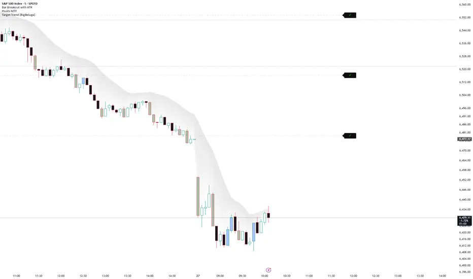
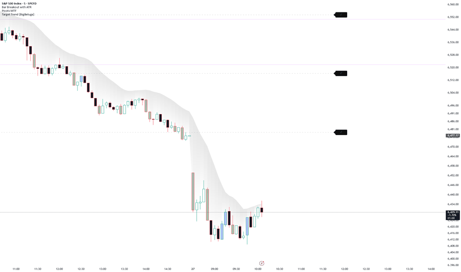
Bar Breakout with ATRBar Breakout with ATR — Multi-Timeframe Dashboard
Identifies high-quality breakout bars across multiple timeframes using a combination of ATR-based range filtering and IBS (Internal Bar Strength) confirmation.
How it works:
A bar is flagged as a breakout when three conditions align simultaneously — the close exceeds the prior bar's high (bull) or undercuts the prior bar's low (bear), the bar's range is at least N× the ATR, and the close quality is confirmed via IBS (top of range for bulls, bottom of range for bears). Bars that are large but fail to break are classified as POSS BULL or POSS BEAR — potential coiling setups worth watching.
Features:
Bar coloring — highlights confirmed breakout bars and large-range non-break bars in distinct colors
MTF Dashboard Table — shows the most recent breakout event (BULL BREAK, BEAR BREAK, POSS BULL, POSS BEAR) across up to 5 user-defined timeframes
Context rows — when the latest event on a timeframe is a POSS BULL/BEAR, the table optionally shows the last confirmed break for directional context
Per-bar detail — each table row displays timestamp (CST), low, high, range (with ATR multiple), midpoint, and IBS value
Fully configurable — ATR length, ATR multiplier, IBS thresholds, colors, table position, font sizes, and per-timeframe toggles
Best used on: Equity index futures (ES, NQ), ETFs, or any liquid instrument where breakout structure and range expansion are meaningful signals. Indicador
Indicador

Indicador

SOXL Breakout# SOXL Breakout — Intraday Breakout Levels & Position Sizing
## What It Does
SOXL Breakout is a day-trading overlay indicator designed for leveraged ETFs (SOXL, TQQQ, etc.) on the **5-minute timeframe**. It automatically plots key price levels each morning and tracks position sizing and P&L across two independent accounts.
## How It Works
Every trading day at **09:25 EST**, the indicator captures the open of that candle and draws three levels:
- **OPEN** — the 09:25 candle's open price (white solid line)
- **TRIGGER** — a configurable percentage above the open (green dashed line, default +1.41%). This is your **buy signal**. When price touches this level during RTH, the indicator enters a simulated long position.
- **STOP LOSS** — a configurable percentage below the trigger (red dashed line, default -8%). If price drops to this level while in a position, the trade is closed at a loss.
### Trade Lifecycle
1. **09:25 EST** — Levels are drawn for the day.
2. **During RTH (09:30–16:00)** — If price hits the TRIGGER, a position is entered at the trigger price. Shares are calculated based on your account size and deploy percentage, rounded down to the nearest 100 shares.
3. **Stop Loss** — If price hits the stop-loss level at any time while in a position (including pre-market the next day), the position is closed.
4. **09:20 EST (next day)** — If still in a position, it is auto-sold at the open price. This is the default exit.
### SOXS (Inverse) Entry
An optional feature for hedging or inverse plays. When enabled, if the TRIGGER was **never hit** during RTH on Monday, Thursday, or Friday, a **SOXS ENTRY** line is drawn at the 15:55 closing price. This signals a potential inverse (bearish) entry.
## The Position Sizing Table
A live overlay table displays:
| Row | Description |
|---|---|
| **Account** | Current account balance (seed + cumulative P&L). Shows before/after transition on trade close. |
| **Running P&L** | Live dollar P&L while in a position, or locked P&L after exit. |
| **Status** | Current state: Waiting, Acct updated, In position, Sold - gain, Sold - loss, Stopped out. |
| **Shares** | Number of shares to trade based on account size, deploy %, and trigger price. |
| **Risk** | Dollar risk and percentage risk per account if stopped out. |
The table supports **two independent accounts** — useful for tracking separate portfolios or different position sizes side by side.
## Settings
### Open Candle Time
- **Open Candle Hour/Minute (EST)** — When to capture the reference candle (default: 09:25)
- **Trigger % above Open** — Percentage above open for the buy trigger (default: 1.41%)
- **Stop Loss % below Trigger** — Percentage below trigger for the stop loss (default: 8.0%)
### Line Colours
- Customize colors for the OPEN, TRIGGER, and STOP LOSS lines.
### SOXS Entry
- **Enable SOXS Entry** — Toggle the inverse entry line feature.
- **SOXS ENTRY colour** — Color for the SOXS entry line.
### Account 1 / Account 2
- **Account Name** — Label shown in the table header.
- **Starting Account ($)** — Your account seed capital. Changing this resets cumulative P&L.
- **Deploy %** — Percentage of account to deploy per trade (default: 80%).
### Display
- **Table Position** — Where to place the position sizing table on the chart.
## Important Notes
- This indicator is designed for the **5-minute timeframe only**. A warning label will appear if applied to any other timeframe.
- Cumulative P&L only updates on **realtime bars** to avoid inflated backtest results.
- Changing the starting account value resets the cumulative P&L counter.
- Shares are always rounded down to the nearest 100.
- The indicator does **not** place actual trades — it is a visual and analytical tool only.
## Disclaimer
This indicator is for **educational and informational purposes only**. It does not constitute financial advice. Leveraged ETFs carry significant risk, including the potential for substantial losses. Always do your own research and consult a qualified financial advisor before trading. Past performance does not guarantee future results.
Indicador

Indicador

Estratégia

Doji Volume Map (Zeiierman)█ Overview
Doji Volume Map (Zeiierman) is a volume reaction scanner that detects doji-like candles appearing with relatively high and rising volume, then converts those events into projected price levels. When a valid signal forms, the script places a bubble on the candle, extends a horizontal reaction level forward, and optionally merges nearby levels into a highlighted zone box. The result is a clean map of potential reaction areas built from high-interest doji events rather than generic swing highs or lows.
⚪ What It Detects
The script searches for candles that combine 3 conditions at the same time:
Relative high volume: Current volume must exceed the average volume by a user-defined multiplier.
Rising volume: Current volume must be greater than the previous bar’s volume.
Loose doji structure: The candle body must remain small relative to the total range, while the full range must still be meaningful enough relative to ATR.
When those conditions align, the candle is treated as a significant reaction point and plotted as a bubble. From there, the script projects the price level forward and can combine overlapping levels into broader zones.
█ How It Works
For each bar inside the Lookback Length, the script checks whether the candle qualifies as a valid signal.
It measures:
Average volume over the selected Volume Average Length
Relative volume strength using the Relative Volume Multiplier
Whether volume is increasing vs the previous bar
Whether the candle body is small enough to be considered doji-like
Whether the total range is large enough relative to ATR
█ How to Use
When a doji-like candle forms with high and rising volume, it signals strong participation but no clear directional control.
This means:
Heavy trading occurred.
Both sides were active.
Price failed to move decisively.
These areas often become key reaction zones, as the market tends to revisit and respond to where significant transactions took place.
⚪ In Trend
In uptrends , signals on pullbacks can act as support/continuation zones
In downtrends, signals on bounces can act as resistance/rejection zones
Focus on using levels in the direction of the trend, where the dominant side is likely to defend.
⚪ In Ranges
Signals near range lows → potential buy/support zones
Signals near range highs → potential sell/resistance zones
Merged zones are especially useful for identifying rotation areas within the range.
⚪ Key Idea
High volume + indecision = high-interest price area
These zones often lead to:
Reactions
Rejections
Or continuation after confirmation
Use retests and price behavior at these levels to guide entries.
█ Settings
Lookback Length — how many bars back the script scans for qualifying signals.
Volume Average Length — baseline used to measure relative volume.
Relative Volume Multiplier — minimum volume expansion required vs average.
Max Body % of Range — defines how small the candle body must be to count as doji-like.
Min Candle Range as ATR Fraction — filters out candles that are too small to matter.
Key effect:
Higher Relative Volume Multiplier = fewer but stronger signals
Lower Max Body % of Range = stricter doji selection
Higher Min Candle Range as ATR Fraction = fewer weak micro-signals
Merge Close Levels Into Box — combines nearby projected levels into a single zone.
Merge Distance (ATR) — controls how close levels must be to merge.
-----------------
Disclaimer
The content provided in my scripts, indicators, ideas, algorithms, and systems is for educational and informational purposes only. It does not constitute financial advice, investment recommendations, or a solicitation to buy or sell any financial instruments. I will not accept liability for any loss or damage, including without limitation any loss of profit, which may arise directly or indirectly from the use of or reliance on such information.
All investments involve risk, and the past performance of a security, industry, sector, market, financial product, trading strategy, backtest, or individual's trading does not guarantee future results or returns. Investors are fully responsible for any investment decisions they make. Such decisions should be based solely on an evaluation of their financial circumstances, investment objectives, risk tolerance, and liquidity needs.
Indicador

Strong Pinbar Reversals MTF | ProjectSyndicateStrong Pinbar Reversals MTF automatically identifies and power-ranks high-probability reversal opportunities by analyzing clusters of institutional pinbar rejections. It filters for quality, calculates a 0-10 strength score for every reversal cluster based on wick purity, cluster density, and candle momentum, and presents all data on the chart and in a comprehensive multi-timeframe dashboard to eliminate noise and focus on reversals that matter.
• 🎯 Power-Ranking System (0-10) — every pinbar cluster is given a strength score based on a strict 5-dimensional algorithm that assesses cluster size, average wick purity, minimum wick purity, candle range versus ATR, and time density, providing an instant quality assessment.
• 🎨 Strength-Based Color Scheme — reversal zones are colored by their power rank; stronger clusters get darker, more prominent colors for immediate visual hierarchy.
• 🧠 Smart Context Detection — automatically ensures that bullish pinbar clusters only fire at local price lows (support) and bearish clusters only fire at local price highs (resistance), completely filtering out fake signals in mid-range consolidation.
• 📊 On-Chart Statistics — each reversal zone displays its direction (Bullish/Bearish) and its calculated strength score directly inside the shaded zone.
• 🧭 Full MTF Dashboard Display — provides a complete market overview across 7 timeframes (M1, M5, M15, M30, H1, H4, D1), showing the latest reversal signal, its strength, entry/SL/TP levels, and how many bars ago it occurred on that timeframe. The dashboard uses persistent state memory, meaning it is perfectly stable and consistent regardless of the chart you are viewing.
• 🔔 Comprehensive Alerts — get notified the moment a new high-strength cluster occurs, with the alert message containing the full details: direction, strength, entry, SL, and TP levels.
• ✅ Quality Control Filters — a user-configurable minimum strength score (default 6.0) allows you to filter out weak, low-probability wicks and focus only on institutional-grade reversal clusters.
• 🔧 Fully Customizable — control everything from the minimum wick percentage and cluster lookback window to the ADR multipliers for universal zone height and SL/TP placement.
• 🎯 Why this algo is unique: Standard pinbar indicators look at single candles and generate massive amounts of false signals in consolidation. This algorithm looks for clusters of rejection (e.g., 3+ pinbars in a tight window) and uses a multi-factor scoring system to quantify the quality of the rejection. It doesn't just show you a wick; it tells you how strong the institutional absorption is. The MTF dashboard provides a complete, stable cross-timeframe perspective that is impossible to achieve with standard single-timeframe indicators.
• 🚀 Apply to Gold (XAUUSD), Forex, Crypto, and Indices on any timeframe. The wick percentage and cluster size settings allow it to adapt to anything from scalping (M1/M5) to swing trading (H4/D1).
• 🎯 How to use this? Focus on trading opportunities from high-strength reversal clusters rated 7/10 or higher, as these show the highest probability of a structural shift. Use the dashboard to quickly identify which timeframes have active rejection zones, and look for alignment between lower timeframe clusters and higher timeframe support/resistance.
• ⚠️ IMPORTANT NOTICE: This indicator is designed to identify high-probability reversal opportunities based on price action rejection. It should NOT be used as a standalone signal for entering trades. Always use it in conjunction with your own trading strategy, market structure analysis, and other technical indicators to confirm trade setups and manage risk. Indicador

8:00-8:15 ORB Retest on 5m Time Frame v1.3 by Alf_AlgoORB Retest on 5m Time Frame
Breakout → Retest → Confirm → Enter
A structured session indicator designed to trade continuation after an opening range breakout using midpoint retests and confirmation.
Opening Range defines session structure
Breakout sets directional bias (with multiple detection modes)
Midpoint retest provides entry location
Momentum confirmation triggers signals
Triple ATR-based TP levels and structure-based SL manage risk
The system avoids chasing breakouts and instead waits for price acceptance and momentum confirmation.
━━━━━━━━━━━━━━━━━━━━━━━━
Timeframe
Pine Script®
Designed exclusively for the 5-minute chart.
The opening range is built using the first three 5-minute candles.
━━━━━━━━━━━━━━━━━━━━━━━━
Opening Range Levels
OR High — upper boundary (teal)
OR Low — lower boundary (red)
OR Midpoint — primary retest level (amber, dashed)
Shaded zone between High and Low for visual clarity
The midpoint acts as the primary retest level for entries.
━━━━━━━━━━━━━━━━━━━━━━━━
Breakout Direction Mode (New in v1.2)
Four modes to determine how directional bias is set after the opening range:
First Break — original behavior; whichever direction breaks out first locks the bias
Last Break — bias updates with each new breakout before the entry window opens, capturing the final sentiment
Strongest Break — the breakout with the largest candle body wins; more conviction = more significant
Directional Preference — manually select Bullish or Bearish; bias is set when the OR locks regardless of price action
For Last Break and Strongest Break modes, triangle markers appear on the chart each time the bias flips, so you can visually track the tug-of-war between bulls and bears before the entry window.
━━━━━━━━━━━━━━━━━━━━━━━━
Bias Logic
Close above OR High → Bullish Bias
Close below OR Low → Bearish Bias
Depending on the selected Breakout Direction Mode, the bias may lock on the first break, update with subsequent breaks, follow the strongest candle body, or be manually chosen.
━━━━━━━━━━━━━━━━━━━━━━━━
Entry Logic
Wait for midpoint retest
Require confirmation
Signal triggers within the active session window
Three confirmation modes are available:
Retest Close Reclaim
Break Retest Candle
Hybrid (default)
━━━━━━━━━━━━━━━━━━━━━━━━
Risk Management — Triple TP System (New in v1.2)
Three take-profit levels are automatically calculated using ATR, all shown on the chart from the moment a signal fires:
TP1 — 2× ATR (default) — solid line
TP2 — 3× ATR (default) — dashed line
TP3 — 5× ATR (default) — dotted line
SL — structure-based, remains fixed throughout the trade
Each TP and SL level gets a label when hit (TP1 ✓, TP2 ✓, TP3 ✓, SL ✗), so you can see exactly where targets were reached or where the stop was triggered. All ATR multipliers are fully adjustable in the settings.
Alert conditions are available for each individual TP hit and SL hit.
━━━━━━━━━━━━━━━━━━━━━━━━
Chart Elements
Opening Range High / Low / Mid with shaded zone
Breakout markers (triangles)
Retest markers (diamonds)
Buy / Sell signal labels
TP1 / TP2 / TP3 and SL levels with hit labels
On-chart dashboard with full state tracking
━━━━━━━━━━━━━━━━━━━━━━━━
Dashboard
The on-chart dashboard displays real-time state:
Session preset
Breakout Direction Mode
First break direction
Current bias
Retest status
Signal status
Confirmation mode
Individual TP1 / TP2 / TP3 and SL hit status
TP ATR multiplier values
━━━━━━━━━━━━━━━━━━━━━━━━
Typical Workflow
Apply on a 5-minute chart
Select your session and breakout direction mode
Allow opening range to form
Observe breakout(s) and bias assignment
Wait for midpoint retest
Enter after confirmation
Monitor TP1 → TP2 → TP3 progression
━━━━━━━━━━━━━━━━━━━━━━━━
v1.2 Release Notes
Added Breakout Direction Mode with four options: First Break, Last Break, Strongest Break, Directional Preference
Added triple take-profit system (TP1, TP2, TP3) with independent ATR multipliers
TP and SL hit labels appear on chart when each level is reached
Added alert conditions for each TP hit and SL hit
Styled OR lines with updated color palette (teal / red / amber)
Added shaded zone between OR High and Low
Updated dashboard with Breakout Direction Mode, individual TP status, and ATR multiplier display
v1.1 Release Notes
Added ORB session selection (New York, London, Asia)
Replaced breakout text labels with directional triangle icons
Replaced retest text labels with diamond icons
Added on-chart dashboard
Dashboard now shows directional state instead of checkmarks
Added Buy / Sell signal display in dashboard
Added color-coded dashboard values (green bullish, red bearish)
Updated Buy/Sell signal label colors
Added TP / SL outcome tracking in dashboard
━━━━━━━━━━━━━━━━━━━━━━━━
Feedback
This script is shared publicly to help traders study structured opening range continuation setups.
Feedback and suggestions are welcome
Ideas for improvements or additional features are appreciated
Indicador

Indicador

Indicador

Indicador

Indicador

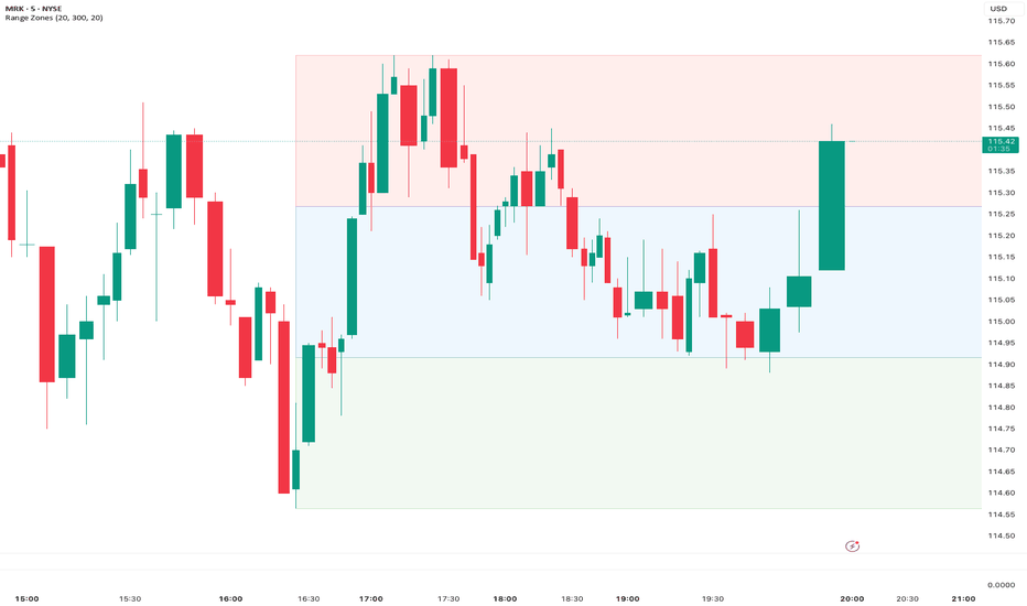
Range Zones AlertsRange Zones — Buy the Green, Sell the Red
Get alerted when price enters a buy zone or a sell zone.
This indicator detects the current trading range, splits it into three color-coded zones, and sends you an alert the moment price touches the zone you care about. No guessing where support and resistance are — the indicator finds them for you.
Green Zone = Buy Zone
The bottom third of the range is shaded green. This is where price has historically found support. When price drops into the green, buyers tend to step in. Set up the Bull alert and get notified the instant price touches this zone — that's your signal to start looking for a long entry.
Red Zone = Sell Zone
The top third of the range is shaded pink/red. This is where price has historically hit resistance. When price pushes into the red, sellers tend to step in. Set up the Bear alert and get notified the instant price touches this zone — that's your signal to start looking for a short entry or to take profits on longs.
Blue Zone = No Trade Zone
The middle third is shaded blue. Price is stuck between support and resistance with no clear edge in either direction. When price is in the blue, wait.
Alerts
Three options in TradingView's alert panel:
— Bull Alert: fires when price touches the green support zone.
— Bear Alert: fires when price touches the red resistance zone.
— Both: fires on either — one alert covers everything.
A built-in cooldown (default 20 bars) prevents spam. You get one alert per zone touch, then silence until the cooldown clears. Bull and bear cooldowns are independent — a green zone alert won't block a red zone alert.
How It Works
The indicator uses pivot-based swing detection to find the most recent significant high and low. The range between them is divided into three equal horizontal zones. The zones update automatically as new swing highs and lows form. A Max Range Age setting ensures stale, outdated ranges are dropped.
Settings
— Pivot Strength: how significant the swing points need to be. Default 20. Higher = wider ranges.
— Max Range Age: how old the range can be before it's dropped. Default 300 bars.
— Alert Cooldown: bars of silence after an alert fires. Default 20.
— Zone Colors: fully customizable.
Works on any ticker, any timeframe. Add it to your chart, set up your alerts, and let the zones tell you when it's time to trade. Indicador
Candle DNA Strand█ CANDLE DNA STRAND
A unique lower-panel indicator that visualizes candle structure as a stylized double-helix pattern. One strand represents body dominance (open-close range) while the other represents wick proportion (shadow-to-body ratio). The strands twist around a center axis with color encoding for bullish/bearish bias, revealing candle character patterns over time in an intuitive DNA-inspired format.
█ CONCEPT
Traditional candlestick analysis focuses on individual candle patterns. The Candle DNA Strand takes a different approach by decomposing every candle into two core metrics and plotting them as intertwined waves:
• Body Strand — Measures how much of each candle is "body" (the filled portion between open and close). High body ratios indicate conviction and directional commitment.
• Wick Strand — Measures how much of each candle is "shadow" (upper and lower wicks combined). High wick ratios indicate rejection, indecision, or failed attempts at direction.
These two strands are phase-offset by 180° to create the classic double-helix DNA appearance. As you scroll through the chart, you can visually identify periods of conviction (body-dominant) versus indecision (wick-dominant), and how candle character evolves over time.
█ HOW IT WORKS
The indicator calculates two normalized ratios for each candle:
Body Ratio = |Close - Open| / (High - Low)
Wick Ratio = (Upper Wick + Lower Wick) / (High - Low)
These ratios are smoothed and then modulated onto sine waves that twist around a center axis at the 50 level. The amplitude of each strand reflects the strength of that metric — larger bodies push the body strand further from center, and larger wicks push the wick strand further out.
The strands are color-coded by the current candle's bias:
• Bullish candles (close ≥ open) → Neon green tones
• Bearish candles (close < open) → Neon red tones
█ TRADE ZONES
The indicator includes an optional Trade Zone detection system based on candle character analysis:
◉ LONG ZONE (Green Background)
Triggers when:
• Average body ratio exceeds the Body Dominance Threshold (default 65%)
• Bullish momentum score > 40% (more bulls than bears in lookback period)
• Average wick ratio below the Wick Rejection Threshold (default 55%)
This identifies periods where price is moving up with conviction — strong bullish bodies with minimal rejection wicks.
◉ SHORT ZONE (Red Background)
Triggers when:
• Average body ratio exceeds the Body Dominance Threshold
• Bearish momentum score > 40% (more bears than bulls in lookback period)
• Average wick ratio below the Wick Rejection Threshold
This identifies periods where price is moving down with conviction — strong bearish bodies with minimal rejection wicks.
◉ CHOP/INDECISION
When the average wick ratio exceeds 60%, the market is showing high rejection and indecision. The DNA strands will show wick dominance during these periods.
Triangle markers appear at zone entry points:
• ▲ Green triangle below the helix = Long zone entry
• ▼ Red triangle above the helix = Short zone entry
█ VISUAL ELEMENTS
DNA Strands
Two intertwined lines representing body and wick ratios, twisting around the center axis with a configurable wavelength.
Base Pair Connectors
Vertical lines connecting the two strands at regular intervals, mimicking the "rungs" of a DNA ladder. These help visualize the spread between body and wick metrics.
Nucleotide Nodes
Small circular markers along each strand showing individual data points.
Fill Zone
Subtle gradient fill between the strands for visual depth. The fill color matches whichever strand is currently on top.
Info Label
Displays current values at the right edge of the chart:
• Current bias (BULL/BEAR)
• Body and Wick percentages
• Active trade zone (if any)
█ PATTERN DETECTION
The indicator automatically detects significant candle patterns based on DNA metrics:
DOJI — Body ratio < 15%
Very small body relative to total range. Indicates indecision.
MARUBOZU — Body ratio > 85%
Almost no wicks. Strong conviction candle with price closing near the high (bullish) or low (bearish).
HAMMER — Wick ratio > 60% with lower wick > 2× upper wick
Long lower shadow showing rejection of lower prices.
SHOOTING STAR — Wick ratio > 60% with upper wick > 2× lower wick
Long upper shadow showing rejection of higher prices.
█ SETTINGS
DNA Helix Settings
• Helix Wavelength — Number of bars for one complete DNA twist cycle (default: 20)
• Helix Amplitude — Vertical spread of the strands from center (default: 35)
• Show Base Pair Connectors — Toggle the connecting rungs (default: On)
• Connector Frequency — Draw a connector every N bars (default: 2)
• Data Smoothing — SMA length for smoothing ratios (default: 3)
• Strand Thickness — Line width for the DNA strands (default: 2)
Trade Zone Settings
• Show Trade Zones — Toggle background highlighting and entry signals (default: On)
• Zone Lookback — Bars to analyze for zone detection (default: 5)
• Body Dominance Threshold — Minimum avg body ratio for zone trigger (default: 0.65)
• Wick Rejection Threshold — Maximum avg wick ratio for zone trigger (default: 0.55)
Fluorescent Colors
• Bullish colors — Neon green and electric green variants
• Bearish colors — Neon red and hot pink variants
• Axis, connector, and zone colors are all customizable
Visual Settings
• Show Nucleotide Nodes — Toggle the small circles on strands (default: On)
• Show Info Labels — Toggle the right-side information label (default: On)
• Show DNA Analysis Table — Toggle detailed analysis table (default: Off)
█ ALERTS
Four alert conditions are available:
1. Long Zone Entry
"Entered LONG zone - strong bullish momentum with conviction candles"
2. Short Zone Entry
"Entered SHORT zone - strong bearish momentum with conviction candles"
3. Doji Pattern
"Doji detected - indecision"
4. Marubozu Pattern
"Marubozu detected - strong conviction"
█ INTERPRETATION GUIDE
Reading the DNA:
When body strand dominates (further from center):
• Market is moving with conviction
• Candles have strong bodies, minimal wicks
• Trend is likely to continue
When wick strand dominates (further from center):
• Market is showing rejection/indecision
• Candles have long shadows relative to bodies
• Potential reversal or consolidation
Strand crossovers:
• When strands cross, character is shifting
• Body crossing above wick → increasing conviction
• Wick crossing above body → increasing indecision
Color consistency:
• Long stretches of green → sustained bullish pressure
• Long stretches of red → sustained bearish pressure
• Alternating colors → choppy, mixed market
█ BEST PRACTICES
1. Use with price context — The DNA strand shows candle character, not direction. Combine with price action on the main chart.
2. Adjust wavelength to timeframe — Shorter wavelengths (10-15) for scalping, longer wavelengths (25-40) for swing trading.
3. Trade zones are filters, not signals — Use zone entries as confirmation for your existing strategy, not as standalone signals.
4. Watch for character shifts — When the dominant strand changes, market behavior is changing. This often precedes reversals.
5. Multiple timeframe analysis — Check DNA character on higher timeframes to understand the broader context.
█ CREDITS
Developed by Hash Capital Research
Pine Script™ v6
This indicator is provided for educational and informational purposes. Always conduct your own analysis and manage risk appropriately. Indicador

Indicador

Statistical Candle Patterns [QuantRegime]## Overview
Most candle pattern indicators just label patterns on your chart. This one goes further — it **backtests every pattern against the actual chart history** and shows you the **real win rate** for each pattern on the specific instrument and timeframe you're trading.
A "Bullish Engulfing" might have a 68% win rate on BTC 4H but only 42% on EUR/USD 15m. This indicator tells you the difference. **Stop guessing which patterns work — measure them.**
## 12 Patterns Detected
| Pattern | Type | What It Signals |
|---------|------|----------------|
| **Bullish Engulfing** | Bullish | New candle fully engulfs previous bearish candle |
| **Bearish Engulfing** | Bearish | New candle fully engulfs previous bullish candle |
| **Hammer** | Bullish | Long lower wick, small body at top — rejection of lows |
| **Shooting Star** | Bearish | Long upper wick, small body at bottom — rejection of highs |
| **Doji** | Neutral | Tiny body — indecision, potential reversal |
| **Morning Star** | Bullish | 3-bar reversal: down → indecision → up |
| **Evening Star** | Bearish | 3-bar reversal: up → indecision → down |
| **Three White Soldiers** | Bullish | 3 consecutive strong green candles |
| **Three Black Crows** | Bearish | 3 consecutive strong red candles |
| **Inside Bar** | Neutral | Current bar fits inside previous bar — consolidation |
| **Bullish Marubozu** | Bullish | Strong green candle with almost no wicks |
| **Bearish Marubozu** | Bearish | Strong red candle with almost no wicks |
## How Win Rates Are Calculated
For each pattern occurrence in the lookback window:
1. Record the close price at the pattern
2. Look forward N bars (default: 5)
3. **Bullish patterns "win"** if the highest high in those N bars > pattern close
4. **Bearish patterns "win"** if the lowest low in those N bars < pattern close
5. Win Rate = wins / total occurrences × 100
This is a real backtest on the actual chart data — not some theoretical "textbook" win rate.
## The Statistics Dashboard
The bottom-right dashboard shows all 12 patterns with:
- **Win %** — Historical win rate on THIS symbol, THIS timeframe
- **Count** — How many times the pattern appeared
- **Type** — Bullish, Bearish, or Neutral
Win rates are color-coded:
- 🟢 60%+ = Strong edge
- 🟡 50-60% = Moderate
- 🔴 Below 50% = Pattern doesn't work here — skip it
## Smart Filtering
Labels only appear on the chart when:
- The pattern has appeared at least N times (configurable, default 3)
- The historical win rate exceeds your threshold (configurable, default 50%)
This means **you only see patterns that have actually worked** on this chart. Low-probability patterns are automatically hidden.
## Key Features
- **12 classic candle patterns** detected automatically
- **Real win rates** calculated from actual chart history — not theory
- **Smart filtering** hides unreliable patterns
- **Full statistics dashboard** with pattern-by-pattern breakdown
- **Customizable detection** — adjust body ratios, wick ratios, lookback windows
- **Toggle individual patterns** on/off
- **11 alert conditions** — one for each pattern type
- **Works on any market, any timeframe**
## Recommended Settings
| Style | Lookback | Outcome Bars | Min Win Rate |
|-------|----------|-------------|-------------|
| Scalping (1-5m) | 200-300 | 3 | 55% |
| Day Trading (15m-1H) | 500 | 5 | 50% |
| Swing (4H-Daily) | 500 | 5-10 | 50% |
| Position (Weekly) | 250 | 3-5 | 45% |
## Important Notes
- Win rates are calculated from historical data and **do not guarantee future results**
- Low occurrence counts (< 5) produce unreliable statistics — increase lookback or use a higher timeframe
- Some patterns (like Doji) are very common — consider raising the min body ratio to filter for higher-quality dojis
- The outcome window matters: 3 bars is aggressive, 10 bars gives more room
- Computing intensive on lower timeframes with high lookback — reduce lookback if the indicator loads slowly
## Disclaimer
This indicator is for educational and analytical purposes only. Past pattern win rates do not guarantee future performance. Always use proper risk management and never rely solely on candle patterns for trading decisions. Indicador

Indicador

Outside Bar & 2-Bar Reversal Alerts + SystemOutside Bar & 2-Bar Reversal — Price Action Reversal Detection with Integrated Trade Management
Hello friends and traders!
🔹 Introduction
This indicator — Outside Bar & 2-Bar Reversal — automatically identifies two of the most structurally sound price action reversal patterns and overlays a complete trade management system directly on your chart.
The patterns this indicator detects are rooted in a simple but powerful idea: momentum exhaustion followed by full absorption. When price makes an aggressive directional push and is then completely engulfed by the opposing side, it often signals that the prevailing move has run out of willing participants.
The indicator also includes an optional suite of confluence filters — VWAP, swing sweeps, and time-of-day — so you can isolate the highest-quality setups rather than trading every signal blindly.
I'll cover the pattern logic, the trade management system, and all filters in detail throughout this description.
🔹 The Premise
🔸 Why Reversal Candles Work
Price moves because of imbalance. When more aggressive buyers than sellers are active, price rises. When more aggressive sellers than buyers are active, price falls.
Reversal candle patterns are useful because they attempt to identify the moment that imbalance flips — where one side that was previously dominant is fully overcome by the other.
The key word is fully. A simple bearish candle after a bullish candle tells you very little. What's meaningful is when the opposing candle completely engulfs the prior move — taking out its low, closing above its open, and reaching above its high. That's not just a pause. That's a statement.
This is the foundation of both patterns this indicator detects.
🔸 What Is an Outside Bar?
An outside bar is a candle that completely engulfs the prior candle — its range exceeds the prior candle's range on both sides.
But not all outside bars are created equal. A random outside bar on a quiet consolidation bar means very little. The patterns this indicator targets require context and directionality before the signal fires.
Bullish Outside Bar — Full Conditions:
Candle 1 must be bearish — it closes below its open
Candle 1 must close below the prior candle's close — a genuine continuation of selling
Candle 1's low must be below the prior candle's low — it must make a lower low, showing directional commitment
Candle 2 (signal candle) must have a lower low than Candle 1 — extending the flush
Candle 2 must close above Candle 1's open — full absorption of the bearish candle
Candle 2 must have a higher high than Candle 1 — completing the engulf
The result: a setup where price made a committed bearish push, and then a single candle came in, swept below it, and closed above the entire prior move. Buyers didn't just show up — they overwhelmed every seller from the prior candle.
Bearish Outside Bar — Full Conditions:
The exact mirror. A committed bullish candle that makes a higher high, followed by a signal candle that sweeps above it and closes below its entire range. Sellers overwhelmed every buyer.
🔸 What Is a 2-Bar Reversal?
The 2-Bar Reversal is a related but distinct pattern. Rather than requiring full range engulfment, it focuses on close-to-close extremity.
Bullish 2-Bar Reversal:
Candle 1 closes entirely below the low of the candle before it — an aggressive, committed flush
Candle 2 closes above the open of Candle 1 — a full reclaim of the prior candle's starting point
The logic: if price closes below a prior candle's entire range, sellers were aggressive. If the very next candle reclaims all of that, buyers responded even more aggressively. The speed of the reversal is what makes this significant.
Bearish 2-Bar Reversal:
Candle 1 closes above the prior candle's high. Candle 2 closes below Candle 1's open. Immediate and full rejection of the breakout.
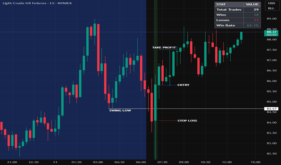
🔹 Integrated Trade Management
Every signal automatically places three levels on your chart so you never have to manually calculate a trade again.
🔸 Entry
The open of the candle immediately following the signal candle. You're not chasing — you're entering at the next structured open after confirmation is complete.
🔸 Stop Loss
The open of the signal candle itself. The reasoning: if price returns to where the signal candle opened, the reversal thesis is structurally compromised.
🔸 Take Profit
Fully user-adjustable R multiple. Default is 2R — meaning for every dollar risked, you're targeting two dollars of reward. Adjustable from 0.1R to any value via the settings panel.
🔸 Line Behavior
All three lines extend to the right in real time and automatically terminate the moment price hits either the TP or SL level. No manual cleanup. No cluttered leftover lines. Every historical trade remains visible on the chart so you can review setups at a glance.
🔹 Live Performance Table
A built-in stats table tracks every closed trade automatically:
Total Trades — all resolved trades
Wins — trades that reached the TP level
Losses — trades that hit the SL level
Win Rate — displayed as a percentage, color coded green above 50% and red below
Load any chart, any timeframe, any market — the table populates in real time and gives you an instant read on how the patterns have performed under your current filter settings.
🔹 Confluence Filters
Each filter is independently toggleable. Use one, all, or none — the indicator works standalone without any filters active.
🔸 VWAP Filter
VWAP (Volume Weighted Average Price) is widely used by institutional participants as an intraday benchmark. Price trading above VWAP is generally considered a bullish market structure for the session; below VWAP is bearish.
When enabled, this filter requires:
Bullish signals: the signal candle must close above VWAP
Bearish signals: the signal candle must close below VWAP
This keeps you aligned with the intraday institutional bias rather than trading reversals against the dominant order flow of the session.
🔸 Swing Sweep Filter
One of the most reliable contexts for a reversal pattern is when it occurs after a liquidity sweep — price briefly trading through a prior swing point before reversing. This is often where stop orders from trapped traders trigger, adding fuel to the reversal.
When enabled:
Bullish signals only show if the signal candle's low swept below a recent pivot low
Bearish signals only show if the signal candle's high swept above a recent pivot high
Both the lookback window and the pivot strength (number of bars required on each side to qualify as a swing) are fully adjustable.
🔸 Time Window Filter
Not all hours of the trading day are equal. The highest-quality price action signals tend to occur during periods of genuine institutional participation — typically the first few hours of the New York session when volume, spread, and volatility are all at their daily peak.
When enabled, signals are restricted to a user-defined time window. Default is 8:00 AM – 11:00 AM EST, covering the New York open. The start and end times are individually adjustable by hour and minute. Uses the America/New_York timezone, so EST/EDT daylight saving transitions are handled automatically.
🔹 Settings Overview
SettingDescriptionShow Bullish / Bearish SignalsToggle each direction independentlyShow Outside BarsToggle OB pattern on/offShow 2-Bar ReversalsToggle 2BR pattern on/offTake Profit R MultipleAdjustable TP target (default 2R)Show Trade LinesToggle entry/SL/TP linesLine ColorsIndependently customizableTime Window FilterOn/off + start/end timeVWAP FilterOn/offSwing Sweep FilterOn/off + lookback + pivot strength
🔹 Works On Any Market & Timeframe
The patterns are purely price-action based — no volume dependency, no indicator inputs. They apply equally to equities, futures, forex, and crypto. Most effective on intraday timeframes (1m–15m) during high-liquidity sessions, but the logic holds on higher timeframes for swing traders as well.
🔹 Closing Remarks
The Outside Bar and 2-Bar Reversal are not new concepts. Traders have been observing these patterns for decades. What this indicator adds is precision in definition — ensuring every signal meets a strict structural checklist rather than firing on any loosely engulfing candle — combined with a fully automated trade management overlay and a real-time performance table.
The filters exist because context matters. The same pattern in the middle of a choppy afternoon session, below VWAP, with no liquidity sweep, is a different proposition to the same pattern at the New York open, above VWAP, after a clean sweep of a prior swing low.
Use the filters to build a ruleset that matches your edge, and use the performance table to validate it.
Drop a comment below with the market and timeframe you're testing this on — always interested to see how different traders apply price action tools. Indicador