Indicador

Indicador

Indicador
Indicador

Indicador

Indicador

Indicador

Indicador

Indicador

Indicador

MTF TMOTMO - (T)rue (M)omentum (O)scillator) MTF (Higher Aggregation) Version
TMO calculates momentum using the DELTA of price. Giving a much better picture of the trend, reversals & divergences than most momentum oscillators using price. Aside from the regular TMO, this study combines four different TMO aggregations into one indicator for an even better picture of the trend. Once you look deeper into this study you will realize how complex this tool is. This version also produce much more information like crosses, divergences, overbought / oversold signals, higher aggregation fades etc. It is probably not even possible to explain them all, there could easily be an entire e-book about this study.
I have been using this tool for a couple of years now, and this is what i have learned so far:
Favorite Time Frame Variations:
1. 1m / 5m / 30m - Great for intraday futures or options scalps. 30m TMO serves as the overall trend gauge for the day. 5min dictates the longer term intraday moves as well as direction of the 1min. 1min is for the scalps. When the 5min TMO is sloping higher focus should be on 1min buy signals (red to green cross) and vice versa for the 5min agg. sloping down.
2. 5m / 30m / 60m - Also an interesting variation for day trading the 3-5 min charts. Producing more cleaner & beginner-friendly signals that lasts couple of minutes instead of seconds.
3. 120m / Day / 2 Day - For the 30m to 1H or 2H timeframes. Daily & 2 Day dictates the overall trend. 120 min for the signals. Great for a multi-day swings.
4. Day / 2 Day / Week - Good for the daily charts, swing trading analysis as the weekly dictates the overall trend, daily dictates the signals and the 2 day cleans out the daily signals. If the daily & 2 day are not aligned togather, daily signal means nothing. Weekly dictates 2 day - 2 day dictates daily.
5. Week / Month / 3 Month - Same thing as the previous variation but for the weekly charts.
TMO Length:
The default vanilla settings are 14,5,3. Some traders prefer 21,5,3 as the TMO length is litle higher = TMO will potenially last little longer which could teoretically produce less false signals but slower crosses which means signals will lag more behind price. The lower the length, the faster the oscillator oscillates. It is the noice vs. the lag debate. The Length can be changed, but i would not personally touch the other two. Few points up or down on length will not drastically change much. But changes on Calc Length and Smooth Length can produce totally different signals from the original.
Tips & Tricks:
1. Observe
- This is the best tip & trick I can give you. The #1 best way to learn how any study operates is to just observe how it works in certain situations from the past. MTF TMO is not
an exception.
2. The Power of the Higher Aggregation
- The higher aggregation ALWAYS dictates the lower one. Best way to see this? Just 2x the current timeframe aggregation = so on daily chart, plot the daily & two day TMOs and you will notice how the higher agg. smooths out the current agg. The higher the aggregation is, the smoother (but slower) will the TMO turn. The real power kicks in when the 3 or 4 aggregations are aligned togather in one direction.
3. Position of the Higher Aggregation in Relation to the Extremes
- Overbought / oversold signals might not really work on the current aggregation. But pay attention to the higher aggregations in relation to the extremes. Ex: on the daily chart - daily TMO inside the OB / OS extremes might not mean much. But once the higher aggregations such as 3 day or Weekly TMO enters OB/OS zone togather with the daily, this can be a very powerful signal for a TMO reversion to the zeroline.
4. Crosses
- Yes, crosses do work. Personally, I never really focused on them. The thing about the crosses is that it is crucial to pick the right higher aggregation to the combination of the current one that would be reliable but also print enough signals. The closer the cross is to the OB / OS extremes, the more bigger move can occur. Crosses around the zero line can be considered as less quality crosses.
5. Divergences
- TMO can print awesome divergences. The best divergences are on the current aggregation (TMO agg. same as the chart) since the current agg. oscillates fast, it can usually produce lower lows & higher highs faster then any higher aggregations. Easy setup: wait for the higher aggregation to reach the OB / OS extremes and watch the current (chart) aggregation to print a divergence.
6. Three is Enough
- I personally find more than three aggregations messy and hard to read. But there is always the option to turn on the 4th one. Just switch the TMO 4 Main, TMO 4 Signal and TMO 4 Fill in the style settings.
Hope it helps. Indicador

Estratégia
Indicador
Indicador

Indicador

Indicador

Indicador
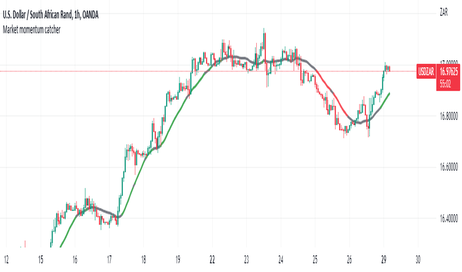
T3 Velocity Candles [Loxx]T3 Velocity Candles is a candle coloring overlay that calculates its gradient coloring using T3 velocity.
What is the T3 moving average?
Better Moving Averages Tim Tillson
November 1, 1998
Tim Tillson is a software project manager at Hewlett-Packard, with degrees in Mathematics and Computer Science. He has privately traded options and equities for 15 years.
Introduction
"Digital filtering includes the process of smoothing, predicting, differentiating, integrating, separation of signals, and removal of noise from a signal. Thus many people who do such things are actually using digital filters without realizing that they are; being unacquainted with the theory, they neither understand what they have done nor the possibilities of what they might have done."
This quote from R. W. Hamming applies to the vast majority of indicators in technical analysis . Moving averages, be they simple, weighted, or exponential, are lowpass filters; low frequency components in the signal pass through with little attenuation, while high frequencies are severely reduced.
"Oscillator" type indicators (such as MACD , Momentum, Relative Strength Index ) are another type of digital filter called a differentiator.
Tushar Chande has observed that many popular oscillators are highly correlated, which is sensible because they are trying to measure the rate of change of the underlying time series, i.e., are trying to be the first and second derivatives we all learned about in Calculus.
We use moving averages (lowpass filters) in technical analysis to remove the random noise from a time series, to discern the underlying trend or to determine prices at which we will take action. A perfect moving average would have two attributes:
It would be smooth, not sensitive to random noise in the underlying time series. Another way of saying this is that its derivative would not spuriously alternate between positive and negative values.
It would not lag behind the time series it is computed from. Lag, of course, produces late buy or sell signals that kill profits.
The only way one can compute a perfect moving average is to have knowledge of the future, and if we had that, we would buy one lottery ticket a week rather than trade!
Having said this, we can still improve on the conventional simple, weighted, or exponential moving averages. Here's how:
Two Interesting Moving Averages
We will examine two benchmark moving averages based on Linear Regression analysis.
In both cases, a Linear Regression line of length n is fitted to price data.
I call the first moving average ILRS, which stands for Integral of Linear Regression Slope. One simply integrates the slope of a linear regression line as it is successively fitted in a moving window of length n across the data, with the constant of integration being a simple moving average of the first n points. Put another way, the derivative of ILRS is the linear regression slope. Note that ILRS is not the same as a SMA ( simple moving average ) of length n, which is actually the midpoint of the linear regression line as it moves across the data.
We can measure the lag of moving averages with respect to a linear trend by computing how they behave when the input is a line with unit slope. Both SMA (n) and ILRS(n) have lag of n/2, but ILRS is much smoother than SMA .
Our second benchmark moving average is well known, called EPMA or End Point Moving Average. It is the endpoint of the linear regression line of length n as it is fitted across the data. EPMA hugs the data more closely than a simple or exponential moving average of the same length. The price we pay for this is that it is much noisier (less smooth) than ILRS, and it also has the annoying property that it overshoots the data when linear trends are present.
However, EPMA has a lag of 0 with respect to linear input! This makes sense because a linear regression line will fit linear input perfectly, and the endpoint of the LR line will be on the input line.
These two moving averages frame the tradeoffs that we are facing. On one extreme we have ILRS, which is very smooth and has considerable phase lag. EPMA has 0 phase lag, but is too noisy and overshoots. We would like to construct a better moving average which is as smooth as ILRS, but runs closer to where EPMA lies, without the overshoot.
A easy way to attempt this is to split the difference, i.e. use (ILRS(n)+EPMA(n))/2. This will give us a moving average (call it IE /2) which runs in between the two, has phase lag of n/4 but still inherits considerable noise from EPMA. IE /2 is inspirational, however. Can we build something that is comparable, but smoother? Figure 1 shows ILRS, EPMA, and IE /2.
Filter Techniques
Any thoughtful student of filter theory (or resolute experimenter) will have noticed that you can improve the smoothness of a filter by running it through itself multiple times, at the cost of increasing phase lag.
There is a complementary technique (called twicing by J.W. Tukey) which can be used to improve phase lag. If L stands for the operation of running data through a low pass filter, then twicing can be described by:
L' = L(time series) + L(time series - L(time series))
That is, we add a moving average of the difference between the input and the moving average to the moving average. This is algebraically equivalent to:
2L-L(L)
This is the Double Exponential Moving Average or DEMA , popularized by Patrick Mulloy in TASAC (January/February 1994).
In our taxonomy, DEMA has some phase lag (although it exponentially approaches 0) and is somewhat noisy, comparable to IE /2 indicator.
We will use these two techniques to construct our better moving average, after we explore the first one a little more closely.
Fixing Overshoot
An n-day EMA has smoothing constant alpha=2/(n+1) and a lag of (n-1)/2.
Thus EMA (3) has lag 1, and EMA (11) has lag 5. Figure 2 shows that, if I am willing to incur 5 days of lag, I get a smoother moving average if I run EMA (3) through itself 5 times than if I just take EMA (11) once.
This suggests that if EPMA and DEMA have 0 or low lag, why not run fast versions (eg DEMA (3)) through themselves many times to achieve a smooth result? The problem is that multiple runs though these filters increase their tendency to overshoot the data, giving an unusable result. This is because the amplitude response of DEMA and EPMA is greater than 1 at certain frequencies, giving a gain of much greater than 1 at these frequencies when run though themselves multiple times. Figure 3 shows DEMA (7) and EPMA(7) run through themselves 3 times. DEMA^3 has serious overshoot, and EPMA^3 is terrible.
The solution to the overshoot problem is to recall what we are doing with twicing:
DEMA (n) = EMA (n) + EMA (time series - EMA (n))
The second term is adding, in effect, a smooth version of the derivative to the EMA to achieve DEMA . The derivative term determines how hot the moving average's response to linear trends will be. We need to simply turn down the volume to achieve our basic building block:
EMA (n) + EMA (time series - EMA (n))*.7;
This is algebraically the same as:
EMA (n)*1.7-EMA( EMA (n))*.7;
I have chosen .7 as my volume factor, but the general formula (which I call "Generalized Dema") is:
GD (n,v) = EMA (n)*(1+v)-EMA( EMA (n))*v,
Where v ranges between 0 and 1. When v=0, GD is just an EMA , and when v=1, GD is DEMA . In between, GD is a cooler DEMA . By using a value for v less than 1 (I like .7), we cure the multiple DEMA overshoot problem, at the cost of accepting some additional phase delay. Now we can run GD through itself multiple times to define a new, smoother moving average T3 that does not overshoot the data:
T3(n) = GD ( GD ( GD (n)))
In filter theory parlance, T3 is a six-pole non-linear Kalman filter. Kalman filters are ones which use the error (in this case (time series - EMA (n)) to correct themselves. In Technical Analysis , these are called Adaptive Moving Averages; they track the time series more aggressively when it is making large moves. Indicador

Indicador

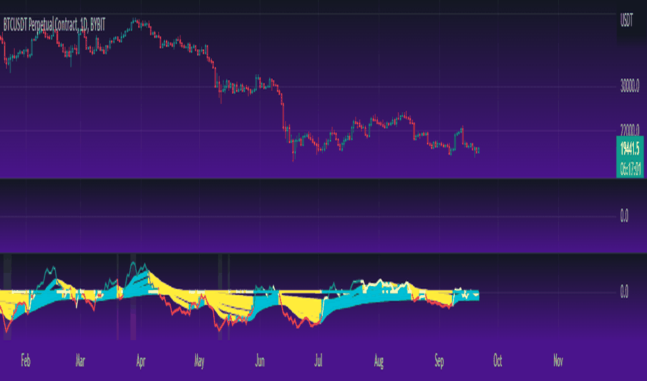
Munich's Momentum Wave V2MUNICH'S MOMENTUM WAVE VERSION 2 IS LIVE!!!
There are a few big things to note with this one.
I decided to upload this as an entirely new script due to the number of changes differing from the first version, but as the last one, this will still work on ANY TIMEFRAME, ANY ASSET CLASS, ANY PRICE! .
This momentum wave indicator now will give you data for when trend could turn, and two momentum indicators to help you decide when to take an entry.
First off,
*I have added an alma ma (alma) that will track momentum alongside price action and further lead the indicator consisting of the Munich waves.
* The background feature will track the price using a method derived from the Bollinger bands, after calculations, it will color the background based on the average of the momentum's ema's, the alma ma, and also the alma in comparison to the alma's value pre offset ( the offset is 3, following the basis).
*There are now 5 basis values given from the increase in ema samples.
If anyone has any questions feel free to pm me or comment below. Thank you guys for the support! :)
INDEX:BTCUSD TVC:NDQ AMEX:SPY BITSTAMP:ETHUSD BINANCE:BTCUSDT FX:USDJPY NASDAQ:AAPL Indicador
Indicador
München's Momentum WaveMUNICH'S MOMENTUM WAVE:
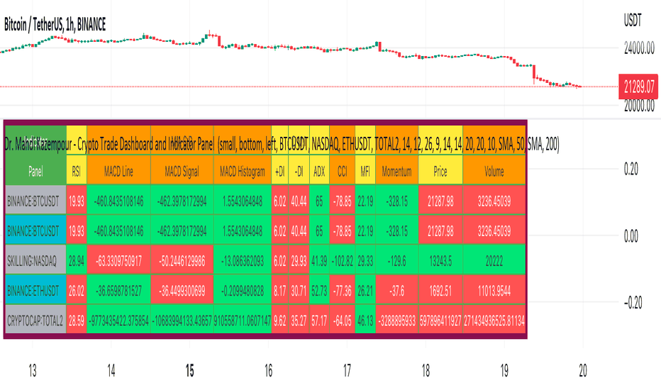
This momentum tracker has features sampled from Madrid's moving average ribbon but has differentiated many values, parameters, and usage of integers. It is derived using momentum and then creates moving averages and mean lengths to help support the strength of a move in price action, and also has the key mean length that helps determine HL/LH or rejections into trend continuation. This indicator works on ALL TIME FRAMES, ALL ASSET CLASSES ON ALL SETTINGS!!
HOW DO I USE IT?
*First off, I have arranged the input settings into groups based on the parts of the indicator it affects.
*You want to use the aqua/white/yellow (Munich's line) as your leading indicator, this is a combined average of the MoM indicator.
* When using Munich's line you want to look at the relation to the mean line (the flat line that adjusts based on price action. You will often see rejections of this line into trend continuation. I personally have caught perfect LH/HL bounce trades off of this indicator.
* Use the Background and other colored moving averages to help pre-determine moves based on the -3 offset value of Munich's line. This was by design not to create 'accurate' results, but to help predict momentum swings based on sharper moves in price action better than if all values lined up to the current bar.
Cheat Code's Notes:
I hope you guys find this indicator to be useful, this is most likely the best indicator that I have written. Simply for the fact it is useful on any chart, any timeframe with any setting. If you guys have any issues with it, shoot me a pm or drop a comment. Thanks!
-CheatCode1
BINANCE:BTCUSDT BITSTAMP:ETHUSD BITSTAMP:BTCUSD PEPPERSTONE:JPYX TVC:DXY TVC:NDQ AMEX:SPY
Indicador

Indicador