NW - Nadaraya-Watson Kernel Regression
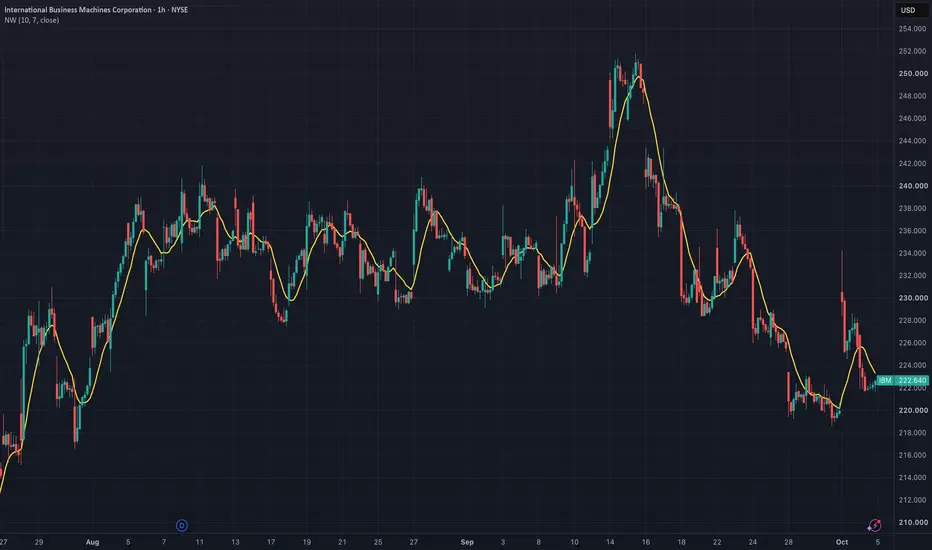
The Nadaraya-Watson (NW) Estimator is a nonparametric regression tool that produces a highly responsive, non-repainting smooth of price data using a Gaussian kernel. Instead of calculating a simple average over a fixed window, it weighs every historical observation in the lookback period by its temporal distance from the current bar. The result is a continuous curve that filters market noise while preserving underlying structural trends, avoiding the abrupt drop-offs seen in traditional moving averages.
HISTORICAL CONTEXT
Elizbar Nadaraya and Geoffrey Watson independently published this kernel regression estimator in 1964. In time-series analysis, the kernel acts as a temporal weighting function.
The NW estimator gained massive popularity on TradingView around 2022. However, most public versions utilize a centered or forward-looking kernel that repaints—meaning the indicator recalculates past values as new price data arrives. While visually perfect in hindsight, repainting indicators are invalid for live trading or backtesting.
This implementation is strictly backward-looking (endpoint mode). The estimate at the current bar relies exclusively on closed historical data. What you see historically is exactly what printed in real-time.
HOW IT WORKS
Stage 1: Gaussian kernel weights
For each historical bar "i" in the lookback window (where i = 0 is the current bar), the weight decays exponentially based on a Gaussian curve.
w_i = exp(−i² / 2h²)
where h is the bandwidth parameter.
Stage 2: Normalized weighted average
The final output is the sum of all weighted prices divided by the sum of all weights.
NW = Sum(w_i × source) / Sum(w_i)
Decay speed and effective window
Weights approach zero rapidly. Observations beyond a lag of 3h bars contribute less than 1.1% of the peak weight.
Setting the lookback window to at least 4h captures over 99.97% of the kernel mass.
INPUTS & PARAMETERS
Bandwidth (h): Dictates the width of the Gaussian bell curve. This is the primary smoothing control.
Lookback Window (Period): The total number of historical bars processed per calculation.
Bandwidth selection
Small h (h << Period): Tight tracking. Weights drop off immediately. Low bias, high variance. Tracks minor noise, prone to whipsaws.
Balanced h (h ≈ Period / 4): Optimal default. Balanced bias and variance. Smooths noise while maintaining trend fidelity.
Large h (h >> Period): Heavy smoothing. Weights remain high across the entire window. High bias, low variance. Flat response.
HOW TO USE
Trend identification
Because it filters out high-frequency noise better than a standard SMA, the NW estimator is highly effective at defining the core directional bias. A rising NW line indicates a structural uptrend, ignoring minor market fluctuations.
Dynamic support and resistance
When paired with standard deviation bands (like Bollinger Bands applied to the NW line instead of an SMA), it creates a highly responsive volatility envelope that doesn't suffer from the "stepping" effect of traditional moving averages.
Crossovers
Using two NW estimators with different bandwidths (e.g., h=8 and h=32) provides a smoother alternative to MACD or EMA crossovers, resulting in fewer false signals during choppy, sideways markets.
LIMITATIONS
Computationally heavy: Requires an O(N) loop iterating through historical data on every single new bar. Very large lookback windows can cause Pine Script execution timeouts.
Inherent Lag (Group Delay): Like all smoothing algorithms, it introduces lag. The group delay is approximately 1.25 × Bandwidth bars.
Cutoff truncation: If the lookback window is set too small relative to the bandwidth (Period < 3h), the Gaussian curve is abruptly cut off, degrading the accuracy of the estimator.
REFERENCES
Nadaraya, E.A. "On Estimating Regression." Theory of Probability and Its Applications, 1964.
Watson, G.S. "Smooth Regression Analysis." Sankhyā: The Indian Journal of Statistics, 1964.
Wand, M.P. & Jones, M.C. Kernel Smoothing. Chapman & Hall/CRC, 1995.
HISTORICAL CONTEXT
Elizbar Nadaraya and Geoffrey Watson independently published this kernel regression estimator in 1964. In time-series analysis, the kernel acts as a temporal weighting function.
The NW estimator gained massive popularity on TradingView around 2022. However, most public versions utilize a centered or forward-looking kernel that repaints—meaning the indicator recalculates past values as new price data arrives. While visually perfect in hindsight, repainting indicators are invalid for live trading or backtesting.
This implementation is strictly backward-looking (endpoint mode). The estimate at the current bar relies exclusively on closed historical data. What you see historically is exactly what printed in real-time.
HOW IT WORKS
Stage 1: Gaussian kernel weights
For each historical bar "i" in the lookback window (where i = 0 is the current bar), the weight decays exponentially based on a Gaussian curve.
w_i = exp(−i² / 2h²)
where h is the bandwidth parameter.
Stage 2: Normalized weighted average
The final output is the sum of all weighted prices divided by the sum of all weights.
NW = Sum(w_i × source) / Sum(w_i)
Decay speed and effective window
Weights approach zero rapidly. Observations beyond a lag of 3h bars contribute less than 1.1% of the peak weight.
Setting the lookback window to at least 4h captures over 99.97% of the kernel mass.
INPUTS & PARAMETERS
Bandwidth (h): Dictates the width of the Gaussian bell curve. This is the primary smoothing control.
Lookback Window (Period): The total number of historical bars processed per calculation.
Bandwidth selection
Small h (h << Period): Tight tracking. Weights drop off immediately. Low bias, high variance. Tracks minor noise, prone to whipsaws.
Balanced h (h ≈ Period / 4): Optimal default. Balanced bias and variance. Smooths noise while maintaining trend fidelity.
Large h (h >> Period): Heavy smoothing. Weights remain high across the entire window. High bias, low variance. Flat response.
HOW TO USE
Trend identification
Because it filters out high-frequency noise better than a standard SMA, the NW estimator is highly effective at defining the core directional bias. A rising NW line indicates a structural uptrend, ignoring minor market fluctuations.
Dynamic support and resistance
When paired with standard deviation bands (like Bollinger Bands applied to the NW line instead of an SMA), it creates a highly responsive volatility envelope that doesn't suffer from the "stepping" effect of traditional moving averages.
Crossovers
Using two NW estimators with different bandwidths (e.g., h=8 and h=32) provides a smoother alternative to MACD or EMA crossovers, resulting in fewer false signals during choppy, sideways markets.
LIMITATIONS
Computationally heavy: Requires an O(N) loop iterating through historical data on every single new bar. Very large lookback windows can cause Pine Script execution timeouts.
Inherent Lag (Group Delay): Like all smoothing algorithms, it introduces lag. The group delay is approximately 1.25 × Bandwidth bars.
Cutoff truncation: If the lookback window is set too small relative to the bandwidth (Period < 3h), the Gaussian curve is abruptly cut off, degrading the accuracy of the estimator.
REFERENCES
Nadaraya, E.A. "On Estimating Regression." Theory of Probability and Its Applications, 1964.
Watson, G.S. "Smooth Regression Analysis." Sankhyā: The Indian Journal of Statistics, 1964.
Wand, M.P. & Jones, M.C. Kernel Smoothing. Chapman & Hall/CRC, 1995.

Rigorous technical indicators for Pine Script 6 with O(1) streaming, defensible math, and proper initialization. Fully documented, implemented in C#, transcribed to Pine Script, and wrapped for Python.
免责声明
这些信息和出版物并非旨在提供,也不构成TradingView提供或认可的任何形式的财务、投资、交易或其他类型的建议或推荐。请阅读使用条款了解更多信息。
Rigorous technical indicators for Pine Script 6 with O(1) streaming, defensible math, and proper initialization. Fully documented, implemented in C#, transcribed to Pine Script, and wrapped for Python.
免责声明
这些信息和出版物并非旨在提供,也不构成TradingView提供或认可的任何形式的财务、投资、交易或其他类型的建议或推荐。请阅读使用条款了解更多信息。