
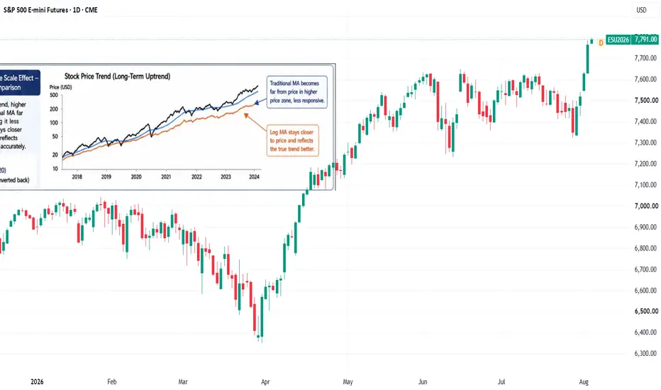
Over the past two weeks, we have introduced two new indicators. However, what I have always hoped is that readers will learn how to improve technical indicators on their own.
In technical analysis, most traditional indicators are calculated directly from price data. For example, a moving average calculates the average closing price, MACD measures trend by comparing the difference between two exponential moving averages, while RSI compares the average gain with the average loss over a specified period.
These methods are simple and straightforward. However, when prices rise substantially over a long period, when different financial instruments trade at vastly different price levels, or when the market experiences extreme volatility, calculations based directly on raw prices may become distorted.

Using LOG, or logarithmic calculations, converts absolute price movements into relative movements. This allows technical indicators to focus more on percentage changes rather than being affected primarily by the absolute price level.
In reality, the market usually cares less about how many dollars a price has risen or fallen and more about the percentage change involved.
One of the greatest advantages of using LOG calculations to improve technical indicators is that they can enhance indicator stability.
Take RSI as an example. A traditional RSI first calculates the price change of each candlestick and then compares the average gains with the average losses.
Suppose a stock rises from $10 to $100. Even if its daily percentage fluctuation remains at 1%, the price movement would initially be only $0.10, while later it would increase to $1. If the calculation is based solely on absolute price changes, the later-period volatility would appear much greater.
An improved method is to replace ordinary price changes with logarithmic returns:
*Log Change = ln(Close ÷ Previous Close)*
Positive values are then treated as gains, while the absolute values of negative changes are treated as losses. The average gain, average loss, and relative strength are subsequently calculated using the original RSI methodology.
The resulting Log RSI will not lose its usefulness simply because the stock price has increased substantially.

The chart above compares traditional RSI with Log RSI. As the stock price rises to increasingly higher levels, traditional RSI may generate overbought signals more easily. However, this is not necessarily reasonable in real-world applications.
Using a Kalman Filter is one way to improve the indicator, while using LOG calculations is another practical approach.
Another advantage of LOG calculations is that they improve comparability across different financial instruments and different time periods.
To put it simply, suppose we want to compare a stock priced at $500, another stock priced at $50, and a futures index quoted at several thousand points.
It is generally impossible to compare all of them fairly using exactly the same indicator and the same set of indicator parameters. This is also a common mistake made by many traders.

Many people assume that the same technical indicator settings should work equally well for stocks, stock index futures, US futures, and other markets. I have never understood why people think this way.
Different products and markets have completely different levels of volatility and price behaviour. How could a day-trading method specifically designed for US stocks be applied directly to stock index futures without modification? That is simply unreasonable.

Many readers have asked me this question over the years. For this reason, our recently introduced Stable Momentum Tracker was designed to be applied across different markets, and LOG calculations are also used as part of its methodology.
Some people may ask whether different products can simply be compared after standardising their price data.
The problem is that if we directly compare the standard deviation of absolute price changes, higher-priced instruments will usually produce larger values. However, this does not necessarily mean that they carry greater risk. The resulting comparison may therefore be misleading.
When volatility is calculated using logarithmic returns, the movements of all instruments are converted to the same percentage-based scale. This allows volatility, momentum, and trading risk to be compared more fairly.
For example, Stock A is priced at $500 and fluctuates by $10 per day, while Stock B is priced at $50 and fluctuates by $2 per day.
At first glance, Stock A appears to be more volatile. However, Stock A is moving by only 2%, whereas Stock B is moving by 4%. In reality, Stock B is the more volatile stock.
The chart above first compares several stocks with different price levels using the standard deviation of absolute price changes. The result may suggest that the highest-priced stock is the most volatile.
However, when the calculation is changed to the standard deviation of logarithmic returns, the true percentage volatility becomes visible, making risk comparisons across different instruments much more meaningful.
LOG calculations can also help reduce misinterpretation.
Suppose a stock rises from $100 to $200. This represents a gain of 100%. If the price subsequently falls from $200 back to $100, the decline is only 50%.
A trader may therefore believe that the stock was much stronger when it rose, while the subsequent decline was not particularly severe because the percentage loss was only “half” of the earlier percentage gain.
This misinterpretation occurs because positive and negative percentage changes are not symmetrical.
When logarithmic returns are used, the two returns become ln(2) and ln(0.5). Their absolute values are identical, with only the direction being different.
This symmetry makes the analysis of compounded returns, statistical models, and technical indicators more consistent.

In practical applications, LOG calculations can be used to improve indicators such as MACD, Bollinger Bands, and ATR.
For MACD, the closing price can first be transformed into ln(Close). The fast EMA and slow EMA are then calculated using the logarithmic price series. The resulting MACD primarily reflects relative trend changes rather than absolute price differences.
For Bollinger Bands, the mean and standard deviation can be calculated using logarithmic prices or logarithmic returns. This reduces the influence of a prolonged high or low price level on the width of the bands.
For indicators such as ATR, traders may divide the true range by the current price or directly calculate the high-low range in logarithmic form. This makes volatility readings more meaningful when comparing instruments with different price levels.
However, LOG calculations also have certain limitations.
The input value must be greater than zero, meaning that logarithms cannot be applied directly to zero or negative values.
If an indicator input may contain negative values, such as a MACD histogram, LOG cannot be applied directly to the completed indicator output.
The correct method is usually to apply LOG to the original price data first and then calculate MACD using the logarithmic price series, rather than calculating MACD first and subsequently applying LOG to the MACD values.
In conclusion, the core value of improving technical indicators with LOG calculations is that it shifts the focus of analysis from “how many dollars the price has moved” to “the proportion or percentage by which the price has changed.”
(Excerpted from our Patreon article)
In technical analysis, most traditional indicators are calculated directly from price data. For example, a moving average calculates the average closing price, MACD measures trend by comparing the difference between two exponential moving averages, while RSI compares the average gain with the average loss over a specified period.
These methods are simple and straightforward. However, when prices rise substantially over a long period, when different financial instruments trade at vastly different price levels, or when the market experiences extreme volatility, calculations based directly on raw prices may become distorted.
Using LOG, or logarithmic calculations, converts absolute price movements into relative movements. This allows technical indicators to focus more on percentage changes rather than being affected primarily by the absolute price level.
In reality, the market usually cares less about how many dollars a price has risen or fallen and more about the percentage change involved.
One of the greatest advantages of using LOG calculations to improve technical indicators is that they can enhance indicator stability.
Take RSI as an example. A traditional RSI first calculates the price change of each candlestick and then compares the average gains with the average losses.
Suppose a stock rises from $10 to $100. Even if its daily percentage fluctuation remains at 1%, the price movement would initially be only $0.10, while later it would increase to $1. If the calculation is based solely on absolute price changes, the later-period volatility would appear much greater.
An improved method is to replace ordinary price changes with logarithmic returns:
*Log Change = ln(Close ÷ Previous Close)*
Positive values are then treated as gains, while the absolute values of negative changes are treated as losses. The average gain, average loss, and relative strength are subsequently calculated using the original RSI methodology.
The resulting Log RSI will not lose its usefulness simply because the stock price has increased substantially.
The chart above compares traditional RSI with Log RSI. As the stock price rises to increasingly higher levels, traditional RSI may generate overbought signals more easily. However, this is not necessarily reasonable in real-world applications.
Using a Kalman Filter is one way to improve the indicator, while using LOG calculations is another practical approach.
Another advantage of LOG calculations is that they improve comparability across different financial instruments and different time periods.
To put it simply, suppose we want to compare a stock priced at $500, another stock priced at $50, and a futures index quoted at several thousand points.
It is generally impossible to compare all of them fairly using exactly the same indicator and the same set of indicator parameters. This is also a common mistake made by many traders.
Many people assume that the same technical indicator settings should work equally well for stocks, stock index futures, US futures, and other markets. I have never understood why people think this way.
Different products and markets have completely different levels of volatility and price behaviour. How could a day-trading method specifically designed for US stocks be applied directly to stock index futures without modification? That is simply unreasonable.
Many readers have asked me this question over the years. For this reason, our recently introduced Stable Momentum Tracker was designed to be applied across different markets, and LOG calculations are also used as part of its methodology.
Some people may ask whether different products can simply be compared after standardising their price data.
The problem is that if we directly compare the standard deviation of absolute price changes, higher-priced instruments will usually produce larger values. However, this does not necessarily mean that they carry greater risk. The resulting comparison may therefore be misleading.
When volatility is calculated using logarithmic returns, the movements of all instruments are converted to the same percentage-based scale. This allows volatility, momentum, and trading risk to be compared more fairly.
For example, Stock A is priced at $500 and fluctuates by $10 per day, while Stock B is priced at $50 and fluctuates by $2 per day.
At first glance, Stock A appears to be more volatile. However, Stock A is moving by only 2%, whereas Stock B is moving by 4%. In reality, Stock B is the more volatile stock.
The chart above first compares several stocks with different price levels using the standard deviation of absolute price changes. The result may suggest that the highest-priced stock is the most volatile.
However, when the calculation is changed to the standard deviation of logarithmic returns, the true percentage volatility becomes visible, making risk comparisons across different instruments much more meaningful.
LOG calculations can also help reduce misinterpretation.
Suppose a stock rises from $100 to $200. This represents a gain of 100%. If the price subsequently falls from $200 back to $100, the decline is only 50%.
A trader may therefore believe that the stock was much stronger when it rose, while the subsequent decline was not particularly severe because the percentage loss was only “half” of the earlier percentage gain.
This misinterpretation occurs because positive and negative percentage changes are not symmetrical.
When logarithmic returns are used, the two returns become ln(2) and ln(0.5). Their absolute values are identical, with only the direction being different.
This symmetry makes the analysis of compounded returns, statistical models, and technical indicators more consistent.
In practical applications, LOG calculations can be used to improve indicators such as MACD, Bollinger Bands, and ATR.
For MACD, the closing price can first be transformed into ln(Close). The fast EMA and slow EMA are then calculated using the logarithmic price series. The resulting MACD primarily reflects relative trend changes rather than absolute price differences.
For Bollinger Bands, the mean and standard deviation can be calculated using logarithmic prices or logarithmic returns. This reduces the influence of a prolonged high or low price level on the width of the bands.
For indicators such as ATR, traders may divide the true range by the current price or directly calculate the high-low range in logarithmic form. This makes volatility readings more meaningful when comparing instruments with different price levels.
However, LOG calculations also have certain limitations.
The input value must be greater than zero, meaning that logarithms cannot be applied directly to zero or negative values.
If an indicator input may contain negative values, such as a MACD histogram, LOG cannot be applied directly to the completed indicator output.
The correct method is usually to apply LOG to the original price data first and then calculate MACD using the logarithmic price series, rather than calculating MACD first and subsequently applying LOG to the MACD values.
In conclusion, the core value of improving technical indicators with LOG calculations is that it shifts the focus of analysis from “how many dollars the price has moved” to “the proportion or percentage by which the price has changed.”
(Excerpted from our Patreon article)

mark chun wai paul
Exención de responsabilidad
La información y las publicaciones no constituyen, ni deben considerarse como, asesoramiento o recomendaciones financieras, de inversión, de trading u otro tipo, proporcionadas o respaldadas por TradingView. Obtenga más información en Condiciones de uso.
mark chun wai paul
Exención de responsabilidad
La información y las publicaciones no constituyen, ni deben considerarse como, asesoramiento o recomendaciones financieras, de inversión, de trading u otro tipo, proporcionadas o respaldadas por TradingView. Obtenga más información en Condiciones de uso.