AXIS BANK | Understanding Gann Square of 9 Degree CompletionEducational Case Study
Disclaimer:
This analysis is for educational purposes only.
I am not a SEBI-registered advisor.
This is not financial advice.
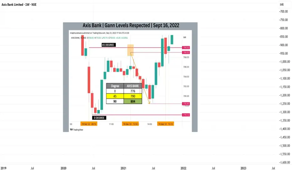
This educational case study explains how the Gann Square of 9 helps identify price–time balance zones, especially in situations where price reaches a key degree level and shows equilibrium instead of immediate reversal.
The purpose of this study is to observe how predefined Gann levels interact with price structure under normal market conditions.
📊 Gann Square Reference Levels
Using standard Gann Square of 9 calculations, the following reference levels were identified in advance:
0° reference level near 658
45° square level near 671
90° square level above the 45° reference zone
These levels represented potential reaction or balance zones, where price could slow down, consolidate, or continue depending on underlying strength.
📈 Observed Market Behavior
Price moved upward from the reference level during the session
Price reached the 45° square level during normal trading hours
Near this level, upward momentum slowed and price began to stabilize
Instead of immediate rejection, price showed temporary balance near the square level
This behavior indicated a phase of equilibrium between buying and selling pressure
This example highlights that Gann levels may act as decision zones, where price can either reverse, consolidate, or continue based on market participation.
🧠 Educational Insight
This case demonstrates important Gann Square of 9 principles:
Gann degree levels help identify potential equilibrium zones
Not all square levels produce immediate directional change
Price stabilization near a degree level can reflect structural balance
Price and time alignment helps traders study market structure objectively
Gann analysis is a framework for observation and discipline, not prediction
Such studies help in understanding how price behaves when interacting with mathematically derived levels.
 Education
Education 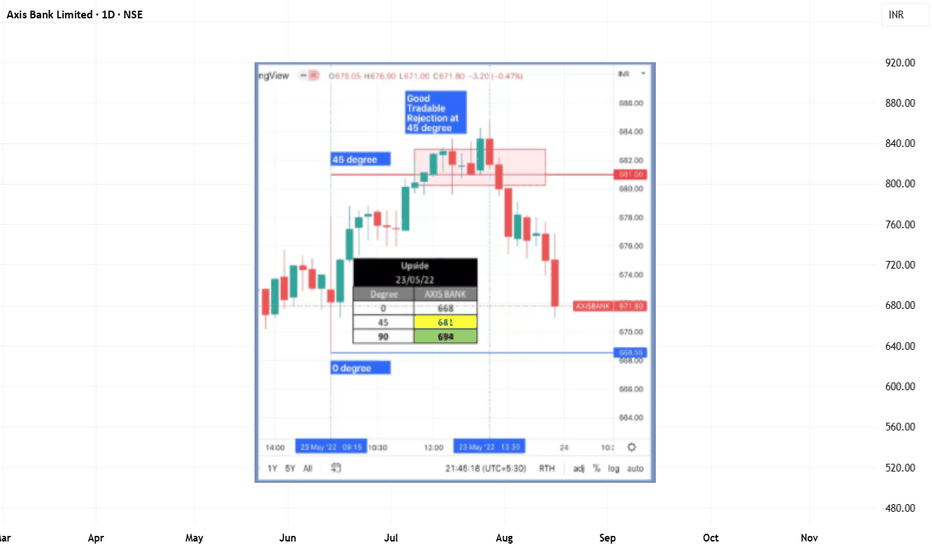
Education 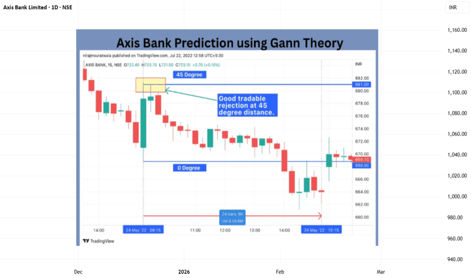
Education 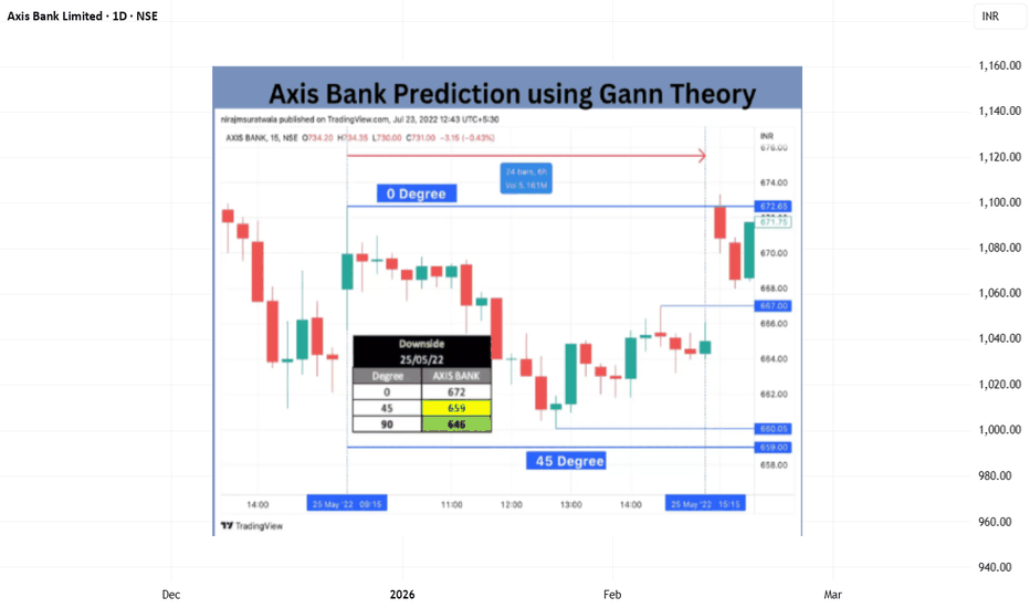
Education 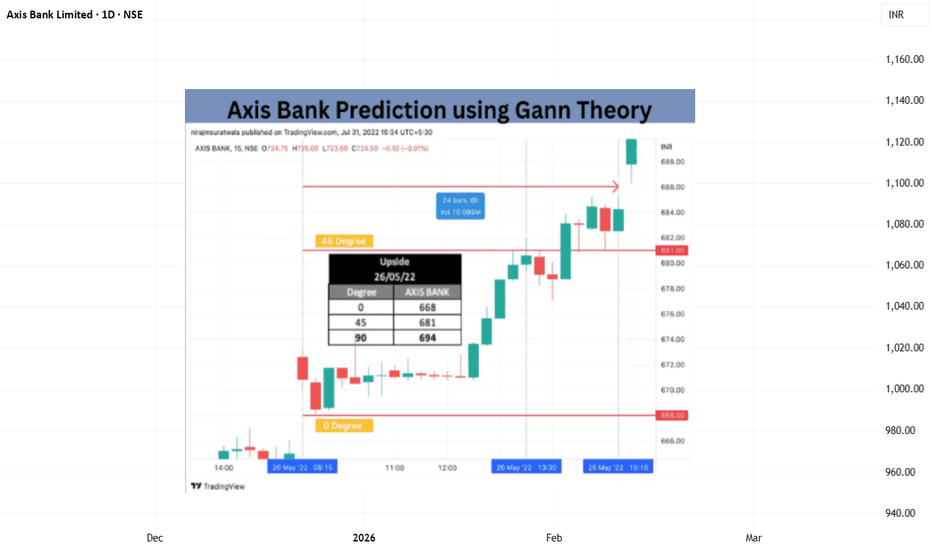
XAUUSD - Wave 5 Expansion or DistributionXAUUSD – Wave 5 Expansion or Distribution Near 5455?
Gold is consolidating around 5340–5360 while geopolitical tension and safe-haven flows continue to dominate headlines.
The US Dollar Index is holding firm near 98.50 as risk sentiment remains fragile due to escalating Middle East conflict. President Trump stated that a “major wave” of attacks against Iran has not yet occurred, leaving uncertainty elevated.
At the same time, ISM Manufacturing PMI came in at 52.4, slightly lower than 52.6 previously but still above expectations (51.8). This suggests the US economy remains stable, supporting the Dollar.
This creates a temporary balance:
Safe-haven demand supports gold.
A stable Dollar caps aggressive upside.
Technical Structure – H1
Gold has completed a clear impulsive sequence and is now transitioning into what appears to be a developing Wave 5 structure.
Key observations:
Strong reaction occurred around the Fibonacci 50% zone (~5250 area).
The 5218 liquidity base remains critical structural support.
Price is now approaching a strong resistance zone near 5375–5400.
Above that sits the major liquidity pool around 5455 (Fibonacci expansion zone).
Momentum is still constructive, but price is now testing supply.
Key Levels
🔹 5218 – Structural Demand
As long as price holds above this zone, bullish structure remains valid.
A breakdown below 5218 invalidates the impulsive continuation scenario.
🔹 5375–5400 – Immediate Resistance
This zone is acting as short-term supply.
Failure here could trigger rotation back toward 5300 or 5250.
🔹 5455 – High Liquidity / Scalping Sell Zone
This is the key magnet above.
If Wave 5 fully expands, this becomes the primary upside objective.
However, this is also where distribution risk increases.
Probable Path
Two scenarios stand out:
Scenario 1 – Wave 5 Extension
Price clears 5400 with momentum → expands toward 5455 liquidity.
This would align with continued geopolitical fear pricing.
Scenario 2 – Short-Term Rotation
Rejection from 5375–5400 → retracement toward 5250–5218 before any further attempt higher.
Given DXY stability near 98.50, aggressive upside may require fresh geopolitical escalation.
Conclusion
Gold is not weak.
But it is approaching a decision zone.
As long as 5218 holds, bullish structure remains intact.
Above 5400, expansion toward 5455 becomes highly probable.
Pay attention to Wave 5 behavior —
late buyers often enter where smart money distributes.
Follow for structured entries — defined risk — and calculated edge.  Long
Long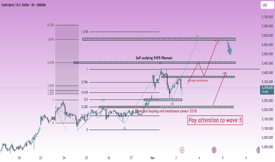
Trade Shapes Global Currency1. Introduction: Trade and Currency Connection
Global trade and global currency markets are deeply interconnected. Every time goods or services cross borders, money must also move across borders. This movement creates demand and supply for different currencies, which directly influences exchange rates. Countries that export more goods than they import tend to see stronger demand for their currency, while countries that import more may experience depreciation pressure.
Trade is one of the most powerful long-term drivers of currency value. Along with interest rates, inflation, and capital flows, trade balances shape how currencies behave in global markets.
2. Trade Balance and Currency Value
The trade balance is the difference between exports and imports.
Trade Surplus: When exports exceed imports
Trade Deficit: When imports exceed exports
For example, when the China exports goods to the United States, American buyers must convert US dollars into Chinese yuan. This increases demand for the yuan.
Impact:
Trade surplus → Higher foreign demand for domestic currency → Currency appreciation
Trade deficit → Higher demand for foreign currency → Currency depreciation
However, this is not always simple because capital flows and monetary policy also influence exchange rates.
3. Export-Led Economies and Currency Strength
Countries that rely heavily on exports often have stronger currencies over time.
Examples:
Germany
Japan
South Korea
These countries export automobiles, electronics, machinery, and technology products globally. Their consistent trade surpluses create steady foreign demand for their currencies.
However, very strong currencies can make exports more expensive. Therefore, some countries try to prevent excessive currency appreciation.
4. Currency Depreciation to Boost Exports
Some nations allow or encourage weaker currencies to make exports cheaper and more competitive globally.
For example:
A weaker Japanese yen makes Japanese cars cheaper internationally.
A weaker Indian rupee makes Indian IT services more attractive globally.
A cheaper currency:
Increases export competitiveness
Reduces imports
Helps correct trade deficits
But depreciation can also increase inflation because imported goods become more expensive.
5. Commodity Trade and Currency Movements
Commodity-exporting countries often have currencies strongly linked to global commodity prices.
Examples:
🇦🇺 Australia
Australia exports iron ore and coal. When commodity prices rise, export income increases, strengthening the Australian dollar.
🇨🇦 Canada
Canada is a major oil exporter. When oil prices rise, the Canadian dollar often appreciates.
Thus, global commodity demand directly shapes these currencies.
6. Trade Agreements and Currency Stability
Trade agreements increase trade volume and reduce uncertainty.
Example:
World Trade Organization promotes free trade.
European Union enables free movement of goods within Europe.
Increased trade integration:
Reduces currency volatility
Encourages long-term foreign investment
Strengthens regional currency blocs
The euro, for example, is supported by strong internal trade within Europe.
7. Current Account and Currency Trends
The current account includes:
Trade balance
Services
Investment income
Transfers
Persistent current account surpluses usually support long-term currency strength. Countries like Japan have maintained strong external balances for decades, supporting their currency stability.
8. Trade Wars and Currency Volatility
Trade conflicts can significantly affect currencies.
Example:
Trade tensions between the United States and China led to volatility in both the US dollar and Chinese yuan.
When tariffs increase:
Export growth slows
Currency may weaken
Investors move capital to safe-haven currencies
Safe-haven currencies include:
US Dollar
Swiss Franc
Japanese Yen
9. Global Supply Chains and Currency Demand
Modern trade operates through global supply chains.
For example:
Raw materials from Australia
Manufacturing in China
Design in the United States
Sales in Europe
Each stage requires currency exchange transactions. Therefore:
High trade integration → High FX market liquidity
More cross-border settlements → Stronger currency interdependence
10. Exchange Rate Regimes and Trade Policy
Countries manage exchange rates differently:
Floating exchange rate (market-driven)
Fixed exchange rate (pegged to another currency)
Managed float (central bank intervention)
For example:
The Chinese yuan is managed by the People’s Bank of China.
The US dollar floats freely in global markets.
Exchange rate policy often aims to support trade competitiveness.
11. Inflation, Trade, and Currency Value
Trade influences inflation, and inflation influences currency.
Strong exports → Higher income → Potential inflation → Currency impact
High imports → Imported inflation if currency weakens
Countries with lower inflation generally have stronger currencies in the long run.
12. Capital Flows vs Trade Flows
In the short term, capital flows (investments, bonds, stocks) can dominate currency movement.
In the long term, trade flows provide fundamental support.
For example:
Foreign direct investment increases demand for domestic currency.
Bond market investments influence exchange rates quickly.
But sustained trade deficits eventually pressure currencies downward.
13. Emerging Markets and Trade Dependency
Emerging markets rely heavily on exports to developed nations.
Example:
India exports IT services and pharmaceuticals.
Brazil exports soybeans and iron ore.
Their currencies are sensitive to:
Global demand
Commodity cycles
US dollar strength
14. Digital Trade and Currency Evolution
With growth in:
E-commerce
Cross-border digital services
Cryptocurrency
Currency dynamics are evolving. Central banks are exploring digital currencies (CBDCs) to simplify cross-border trade settlements.
15. Conclusion: Trade as a Structural Currency Driver
Trade shapes global currency in multiple ways:
Determines demand and supply of currencies
Influences trade balance and current account
Impacts inflation and economic growth
Connects commodity cycles to currency values
Drives exchange rate policy decisions
In the short run, speculation and capital flows dominate.
In the long run, sustained trade patterns determine currency strength or weakness.
Global trade is not just about goods and services — it is the foundation of global currency valuation.  Education
NIFTY – March 2026 Time Structure Outlook(Educational Time-Cycle Study)
March will not be about speed.
It will be about timing.
Not every candle matters.
But certain dates do.
For March 2026, two Time clusters stand out clearly on the structure:
🔶 Cluster 1: 4 – 6 March 2026
🔶 Cluster 2: 16 – 20 March 2026
These are not prediction dates.
They are observation windows.
Time is where price tends to reveal intent.
Current Structural Context
Nifty has been compressing within a broader corrective rhythm.
If weakness extends into the first cluster window,
I will closely observe reaction near the following structural zones:
• 24,790
• 24,545
• 24,390
These are not random numbers.
They are vibration levels derived from prior swing symmetry and time–price alignment.
If Nifty approaches this band during Cluster 1 and stabilizes —
an interim bottom formation becomes possible.
If that happens,
a reversal attempt could unfold into the second cluster (16–20 March).
But Time must confirm.
Price alone does not decide.
Risk Structure – Critical Observation
Markets are not emotional.
They are mathematical.
If we see any sustained daily / 3-day closing below 24,930,
the structure weakens significantly.
In that case, lower expansion zones open:
• 23,515
• 22,782
• 21,926
These levels would represent structural recalibration —
not panic.
Time expands when structure fails.
How I Approach These Windows
I do not anticipate.
I observe.
Around these cluster dates, I will monitor:
• Volatility expansion
• Closing strength vs intraday rejection
• Volume behavior near key levels
• Angle defense / breakdown
Only reaction within the window matters.
Outside of Time, noise dominates.
Inside Time, intention reveals itself.
Final Note
This is a Time-Structure study, not certainty.
No buy.
No sell.
No trade call.
Only mapped windows and defined risk.
Most traders react to movement.
Structured traders prepare for dates.
📐 Time > Price
Educational study only.
Not investment advice.
#LTTSThe Breakdown: After spending much of 2025 consolidating between 3,900 and 4,900, the stock has recently plunged below the critical support level of 3,908.00 (marked in red).
Price Discovery: The stock is currently trading at 3,512.40, gaining 3.41% in the latest week. While this gain is a relief, the price is still significantly below the previous floor, meaning the 3,900 level will likely now act as a stiff resistance (the "support-turned-resistance" principle).
Target Zones: If the current minor bounce fails, the next visible support areas on the historical chart would be near the 3,250 mark. BRIAN XAUUSD – Liquidity map influencing global marketsBRIAN XAUUSD – LIQUIDITY MAP DRIVING GLOBAL GOLD VOLATILITY
On the H2 timeframe, XAUUSD is still holding a bullish structure (higher highs and higher lows), but price is entering a sensitive zone: major liquidity sits overhead, while a wide value/demand area sits below. When price approaches these liquidity pools, volatility typically expands because larger participants often “sweep liquidity first, trend later.”
What’s influencing global gold swings right now
Gold tends to move sharply when expectations around interest rates and the US dollar shift. Any information that forces the market to reprice inflation, yields, or the policy outlook can trigger a liquidity run. From a price-action perspective, the impact is rarely about whether the news is “good or bad” — it’s about which liquidity area price is driven into first, where orders get absorbed and the next directional move forms.
Liquidity structure on the chart
1) Overhead sell-side liquidity
The sell-side liquidity zone above is a natural upside magnet for the current bullish leg. If structure remains intact and the market continues to accept higher prices, price often pushes up to sweep this area before printing a meaningful pullback.
2) Key demand/value zone
The 4,860–4,910 area is the critical demand/value support zone. This is where strong absorption is most likely if a deeper correction unfolds. If price returns to this zone and holds, the probability of a base forming and the uptrend resuming becomes significantly higher.
3) Lower buy-side liquidity
The lower buy-side liquidity area (near the deeper lows) becomes relevant only if bullish structure breaks decisively. If price loses the demand zone and fails to reclaim it, downside acceleration is possible as price moves through thinner liquidity.
Trading scenarios
Scenario 1: Bullish continuation, sweep overhead liquidity
Condition: price maintains bullish structure and does not lose the key demand zone.
Expectation: a push higher to sweep overhead liquidity, followed by a technical pullback.
Scenario 2: Pullback into 4,860–4,910, then bullish rotation
Condition: price corrects into 4,860–4,910 and shows a clear hold.
Plan: prioritize watching for absorption/rotation signals in this zone to re-align with the broader trend.
Scenario 3: Structure failure, deeper downside rotation
Condition: price breaks below 4,860–4,910 and is rejected on a retest from below.
Expectation: a distribution/deeper correction phase towards lower liquidity.
Conclusion
This liquidity map suggests gold is being pulled between two extremes: an upside sweep into overhead liquidity if structure holds, and the 4,860–4,910 demand zone as the decision point if a correction develops. When news increases volatility, the market often runs into these liquidity pools first before confirming the next trend phase.
Follow the Brian channel for daily XAUUSD liquidity levels, scenarios, and structure-based trade plans. Long 
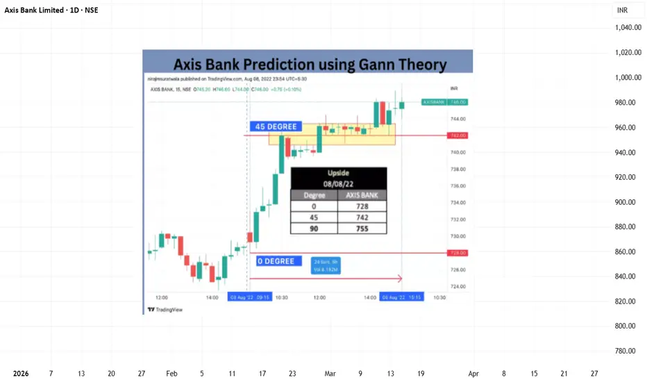
Axis Bank | Gann Square of 9 Observation | Intraday Study Disclaimer:
This analysis is for educational purposes only. I am not a SEBI-registered advisor. This is not financial advice.
Symbol: AXISBANK (NSE)
Date Observed: 08 August 2022
Time Frame: 15-Minute Chart
Concept Studied: Gann Square of 9 (Price–Degree Levels)
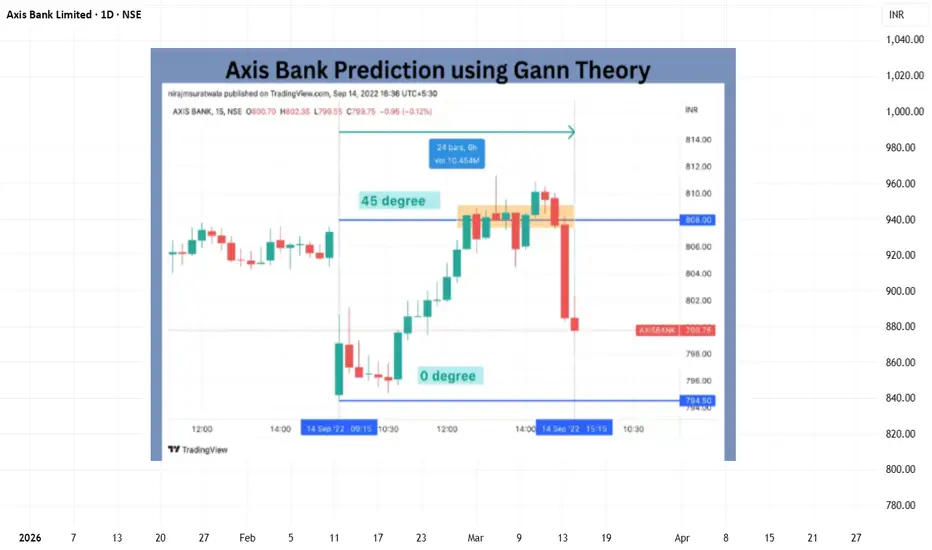
This idea presents a historical intraday observation of Axis Bank using the Gann Square of 9 framework to study how price behaved around calculated degree levels.
The purpose is to demonstrate how Gann levels may act as structured reference zones where price can pause, consolidate, or change behavior depending on market conditions.
📊 Reference Point and Key Gann Levels
During this session, Axis Bank initiated an upward move from a level near 728, which was treated as the 0-degree reference point.
Using price-to-degree conversion, the following levels were observed:
0 Degree: ~728
45 Degree: ~742
90 Degree: ~755
These levels represent mathematically derived zones that can help study market structure objectively.
⏱️ Observed Intraday Price Behavior As the session developed:
Price advanced steadily toward the 45-degree zone (~742)
This level was reached before the late-session time window
Around this zone, the market showed temporary balance and sideways movement
Instead of an immediate directional move, price remained near this level for an extended period
This type of behavior suggests that Gann levels may act as equilibrium zones, where momentum can slow or transition.
📘 Educational Insights: Understanding Gann Levels
Gann levels represent structured price zones derived from mathematical relationships
These levels may function as potential reaction zones, not guaranteed reversal points
Market response may appear as reversal, consolidation, or continuation
Time and price alignment both influence how price behaves at these levels
Not every level produces strong movement, highlighting the importance of observation and discipline
This example demonstrates how Gann levels can be used to study intraday structure using objective and repeatable methods.
#AxisBank #GannSquareOf9 #WDGann #IntradayStudy #TechnicalAnalysis #MarketStructure #TradingEducation
Education 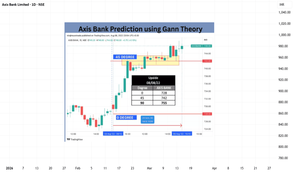
Education 
Global IPO (Initial Public Offering) Trends📊 1. Global IPO Market Overview (2024–2025)
After a multi-year slump following the 2021 peak — when IPO fundraising hit record levels — the global IPO market has shown mixed signals of recovery and recalibration.
According to the EY Global IPO Trends 2025 report, global IPO activity stabilised in 2025, with 1,293 listings raising around US $171.8 billion, reflecting a strong 39 % increase in proceeds compared with 2024. This suggests issuers are focusing more on quality and size over sheer volume.
However, earlier in 2025, some data showed that the total number of IPO transactions had not fully rebounded — although proceeds climbed, indicating larger individual deals and fewer smaller ones.
📉 Contrasting Trends
In mid-2025, Reuters reported a slump in global IPO activity, with volumes falling to their lowest in nine years, driven by trade tensions, volatility and higher costs of capital. In that period, U.S. and European activity fell sharply, though Asia-Pacific saw gains.
Yet, other datasets pointed to resilience and growth, with the first half of 2025 showing robust proceeds and cross-border listings rising.
This juxtaposition highlights that the IPO market, while recovering, remains uneven and sensitive to macroeconomic forces.
🌍 2. Regional Breakdown: Asia, U.S. & Europe
🇮🇳 India: Fastest-Growing IPO Hub
One of the most striking shifts in the global IPO landscape has been India’s rise:
India led the world in IPO volume in 2025, with 367 listings and US $22.9 billion raised, accounting for nearly a third of all global IPO deals.
The country’s capital markets have become a dominant force both in mainboard and SME segments, with high retail and institutional participation. India even led global IPO volumes in specific months, outranking major markets like the U.S. in sheer deal count.
This surge reflects broader economic growth, regulatory reforms, an expanding investor base, and companies increasingly tapping public markets for growth capital.
🇺🇸 United States: Proceeds Leader, Volume Steady
While not leading in volume, the U.S. continues to command the highest IPO proceeds globally:
In 2025, U.S. IPO fundraising outpaced all other markets in dollar terms, driven by larger individual deals and deep investor pools.
The U.S. market has seen notable tech and fintech listings, though performance has been mixed; many 2024–2025 tech IPOs have traded sideways or below IPO prices post-listing, dampening enthusiasm somewhat.
🏙 Hong Kong & China: Strategic Resurgence
Hong Kong — historically one of the world’s most active IPO hubs — has experienced a renewed surge:
A combination of eased regulations and increased Chinese company listings boosted Hong Kong’s IPO activity in 2025, positioning it to potentially reclaim its leadership role.
Major companies, including Swiss-based multinational Syngenta, have eyed Hong Kong for large offerings of up to US $10 billion, underscoring the exchange’s global relevance.
However, broader Chinese mainland IPO volumes remain sensitive to regulatory policy and broader economic headwinds, leading many companies to choose alternative listing venues.
🇪🇺 Europe: Lower Activity, Selective Strength
IPO activity in Europe has generally lagged behind Asia and North America in recent years, partly due to geopolitical uncertainty and regional economic headwinds. European markets have seen fewer large IPOs, though the regulatory environment in the UK and other European centres continues to evolve with initiatives aimed at revitalising listings.
📈 3. Sectoral Patterns & Market Themes
💡 Technology & Innovation
Technology remains a magnet for IPO capital, despite market volatility:
AI-related startups, high-growth cloud and software firms, and fintech companies remain high on investor watchlists, with some envisaged blockbuster listings in 2026.
Tech IPOs often attract speculative interest — and also notable post-listing volatility — highlighting both growth potential and risk.
🧬 Healthcare & Biotech
Healthcare and biotech have maintained IPO relevance:
Companies like Generate Biomedicines aim for multi-billion dollar IPOs, reflecting ongoing investor appetite for innovative healthcare technologies.
⚡ Energy & Clean Tech
Clean energy and sustainability-linked firms are increasingly seeking public capital:
Clean Max Enviro Energy Solutions’ IPO in India drew significant institutional interest, even though retail subscription lagged — reflecting mixed investor interest but growing importance of ESG-aligned offerings.
📊 4. IPO Market Drivers & Challenges
🧭 Drivers of Recent IPO Growth
Market Stabilisation & Investor Confidence – Central banks loosening monetary conditions and easing volatility have helped rekindle IPO interest.
Sector Innovation – Tech, fintech, healthcare, and sustainability sectors continue to produce IPO-ready firms.
Emerging Market Momentum – India and parts of Asia are now driving a significant share of global IPO volume.
Cross-Border Listings – A growing number of companies choose markets outside their home country to access broader capital pools.
🚧 Challenges Facing the IPO Market
Volatility & Geopolitical Risk – Trade disputes, inflationary concerns, and geopolitical tensions make pricing and timing IPOs difficult.
Market Liquidity Concerns – Pullbacks in tech valuations have dampened enthusiasm for riskier IPOs, with some companies postponing or cancelling plans.
Performance Post-Listing – Many IPOs trade below their offer price shortly after listing, which can erode investor confidence over time.
🔮 5. What’s Ahead for IPOs (2026 & Beyond)
The near-term IPO pipeline remains strong, with several blockbuster candidates expected to debut in 2026, including major tech and AI firms. Continued economic recovery and technological innovation are likely to fuel future public offerings.
Key future considerations:
Will Asia, particularly India and Hong Kong, continue to gain share in the global IPO pie?
Can the U.S. maintain leadership in proceeds with marquee tech listings?
How will regulatory shifts in Europe and emerging markets impact issuers’ listing choices?
How will investor sentiment evolve as post-IPO performance trends become clearer?
📌 Summary
The global IPO landscape is in flux but showing resilience. After a downturn following record levels in 2021, markets are recalibrating with a mix of strong proceeds, evolving regional leadership (notably India’s rise and Asia’s strength), and heightened focus on larger, quality offerings. While volatility and macro risks persist, the IPO market’s recovery underscores the enduring role of public capital in corporate growth and investor portfolios.
If you’d like, I can provide a shorter summary or a visual trend chart — just let me know!  Education
Education 
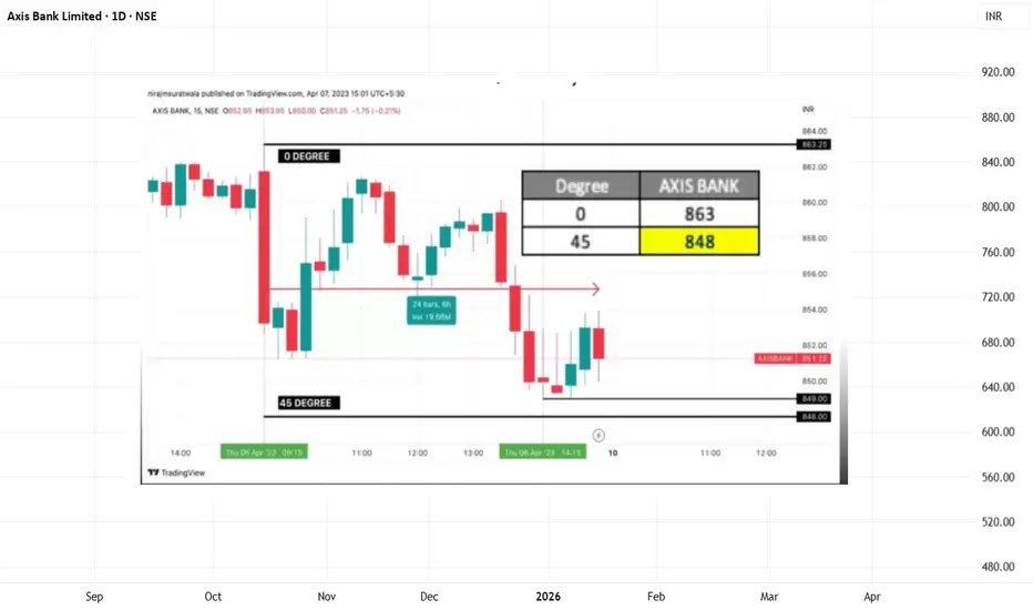
Axis Bank | Gann Square of 9 Intraday Observation | 06/04/2023Disclaimer:
This analysis is for educational purposes only. I am not a SEBI-registered advisor. This is not financial advice.
Symbol: AXISBANK (NSE)
Date Observed: 06 April 2023
Time Frame: 15-Minute Chart
Concept Studied: Gann Square of 9 (Price–Degree Analysis)
This idea highlights an intraday observation of Axis Bank using the Gann Square of 9 framework to study how price behaved near calculated degree levels and how time and price alignment influenced market structure.
📊 Reference Point and Calculated Levels
During this session, Axis Bank initiated a downward move from a level near 863, which was treated as the 0-degree reference point for analysis.
Using Square of 9 conversion, the following level was observed:
0 Degree: ~863
45 Degree: ~848
These calculated levels represent structured zones where the market may show pause, consolidation, or temporary shift in direction based on historical price behavior.
⏱️ Intraday Price Behavior and Reaction As the session progressed:
Price gradually moved downward toward the calculated 45-degree zone
Around 14:15, the market reached a low near 849, which was very close to the observed 45-degree level
Near this zone, price showed temporary stabilization and upward movement
The upward move continued modestly, reflecting a limited intraday recovery
Such reactions near calculated degree levels are commonly observed and may indicate areas where price temporarily balances before the next move develops.
📘 Educational Observations
Gann Square of 9 helps define measured price zones for structured observation
These levels should be viewed as potential reaction zones, not guaranteed reversal points
Minor variation around calculated levels is part of normal market behavior
Time of arrival at a degree level may influence how price responds afterward
Not all reactions lead to large moves, which highlights the importance of disciplined observation
This example demonstrates how Gann-based price-degree analysis can be used to study intraday market structure in an objective and rule-based manner.
#AxisBank #WDGann #GannSquareOf9 #IntradayObservation #TechnicalEducation #PriceTimeAnalysis #MarketStructure
Education 
Today's Gold Price Target: $5260Today's Gold Price Target: $5260
1. The current gold price is around $5190, a crucial level.
Yesterday, gold attempted to break through $5200 again but ultimately retreated, indicating heavy upward pressure.
Meanwhile, new developments in the US-Iran negotiations, which are captivating the market, have further complicated the situation.
2. With the $5200 level proving difficult to breach, market sentiment is cautious, and several institutions have warned of a short-term pullback risk. Therefore, today's strategy could consider shorting at higher levels, but primarily focusing on buying at lower prices.
3. Key Intraday Price Levels
Support Levels:
First support level to watch: $5140-$5150;
If this level breaks, stronger support lies around $5100-$5120.
Resistance Levels:
The first resistance level is the $5195-$5200 mark;
If this level is unexpectedly broken, the next resistance level is in the $5215-$5222 / $5260-$5300 range.
4: Follow-up Developments in US-Iran Talks
After yesterday's third round of talks, no final agreement was reached, but both sides released positive signals. Oman, the mediator, stated that the talks had made "significant progress," and the Iranian Foreign Minister also indicated that they were "close to reaching a consensus" in some areas.
Both sides have agreed to hold technical-level talks in Vienna next Monday (March 2nd).
Impact on Gold Prices:
Short-term negative: Progress in the talks and the agreement to continue negotiations significantly reduced the risk of an immediate military conflict.
Market risk aversion has therefore eased, which is one of the important reasons why gold prices fell back after breaking through $5200 yesterday.
As long as the negotiations do not break down, this factor will continue to put pressure on gold prices.
5. Today, the US will release two crucial data points for the Federal Reserve's monetary policy: the January core PCE price index and the January personal spending month-on-month rate.
Core Logic: PCE is the Fed's preferred inflation indicator.
If the data shows inflation remains stubborn (higher than expected), it could weaken market confidence in a Fed rate cut this year, thus boosting the dollar and suppressing gold prices.
Conversely, weak data would strengthen expectations of a rate cut, benefiting gold prices.
Tonight's US inflation data will be key to determining whether gold prices will find support downwards or break out upwards.
Current Strategy: (Buy on dips, wait for a breakout)
As shown in the chart:
BUY: 5180-5190
SL1: 5130-5150
SL2: 5120-5100
TP: 5250-5300-5400 Understanding Global Market RiskIntroduction
Global market risk refers to the potential for investors, companies, and economies to incur financial losses due to adverse changes in the global financial environment. Unlike local or domestic risks, which are confined to a particular country or market, global market risks stem from interconnected international economic, political, and financial dynamics. These risks are especially relevant in today’s world, where globalization, technology, and cross-border capital flows have tightly linked economies and financial markets.
Investors, multinational corporations, governments, and financial institutions all face global market risk. It can manifest in multiple forms, including currency fluctuations, interest rate changes, commodity price volatility, geopolitical tensions, and systemic financial crises. Understanding and managing these risks is critical for long-term financial stability and effective investment decision-making.
Types of Global Market Risk
Market Risk (Systematic Risk):
Market risk represents the exposure to losses due to broad movements in financial markets. It is systematic because it affects all assets in some form and cannot be eliminated through diversification. For instance, a global recession can simultaneously lower stock prices worldwide, impact bond yields, and reduce commodity demand. Within market risk, there are key subcategories:
Equity Risk: The risk that stock prices decline due to macroeconomic or political events.
Interest Rate Risk: The possibility that bond prices fall or borrowing costs rise when global interest rates change.
Commodity Risk: Exposure to fluctuating prices of essential commodities like oil, gold, or agricultural products.
Currency Risk (Foreign Exchange Risk):
Multinational companies and investors operating across borders face currency risk due to exchange rate volatility. For example, a U.S.-based investor holding European stocks may experience gains or losses not just from the stock price movements but also from changes in the euro-to-dollar exchange rate. Currency risk can affect profits, balance sheets, and investment returns and is often amplified in emerging markets.
Credit and Counterparty Risk:
Global market risk also encompasses the possibility that foreign governments, banks, or corporations may default on their obligations. Sovereign debt crises, such as the European debt crisis of the early 2010s, illustrate how interconnected financial systems can propagate losses globally. Similarly, a major bank default can trigger cascading effects across international markets.
Liquidity Risk:
Liquidity risk arises when investors or companies cannot buy or sell assets quickly without affecting the asset’s price. During periods of global financial stress, markets can freeze, making it difficult to convert investments into cash. For example, during the 2008 global financial crisis, even high-quality assets became illiquid, magnifying losses.
Geopolitical and Political Risk:
Political instability, wars, sanctions, and trade disputes can create sudden and severe disruptions in global markets. For instance, trade tensions between major economies like the United States and China can impact commodity prices, disrupt supply chains, and create uncertainty in global equity and bond markets.
Regulatory and Policy Risk:
Changes in international regulations, taxation policies, or monetary policies by major central banks affect global liquidity and investment flows. Decisions by the U.S. Federal Reserve or the European Central Bank regarding interest rates, quantitative easing, or capital controls can have a ripple effect on global financial markets.
Sources of Global Market Risk
Economic Cycles and Recessions:
Global markets are influenced by economic booms and busts. A slowdown in major economies can reduce demand for exports, decrease corporate profits, and negatively affect stock and bond markets worldwide.
Globalization and Interconnectedness:
While globalization allows capital to flow freely across borders, it also means that shocks in one market can quickly spread to others. For example, a financial crisis in a major economy like the U.S. or China can impact emerging markets, commodities, and currency stability globally.
Technological Disruption:
Rapid technological advancements can create both opportunities and risks. While innovations in fintech, AI, and automation drive growth, they also introduce systemic risks, such as cyberattacks, algorithmic trading failures, and sudden market dislocations.
Natural Disasters and Climate Risk:
Extreme weather events, pandemics, and climate change can disrupt supply chains, affect commodity prices, and cause sudden market volatility. The COVID-19 pandemic is a prime example, as it triggered a global market sell-off, highlighting the vulnerability of markets to non-economic shocks.
Investor Behavior and Market Sentiment:
Global markets are also influenced by psychology and herd behavior. Panic selling, speculation, and over-leveraging can exacerbate price swings and amplify market risks.
Measuring and Managing Global Market Risk
Financial institutions, governments, and investors employ various tools to measure and mitigate global market risk:
Value at Risk (VaR):
VaR estimates the maximum potential loss over a specified period at a given confidence level. It provides a quantifiable metric for global market exposure.
Stress Testing and Scenario Analysis:
These tools simulate extreme market conditions to assess the resilience of portfolios, institutions, or economies to shocks like interest rate spikes, currency devaluations, or geopolitical crises.
Diversification:
Spreading investments across geographies, asset classes, and industries helps reduce exposure to any single source of risk. While diversification cannot eliminate systematic global risk, it can mitigate its impact on individual portfolios.
Hedging Strategies:
Investors and corporations use derivatives such as futures, options, and swaps to hedge against currency, interest rate, and commodity risks.
Regulatory Safeguards:
Governments and international bodies (e.g., the International Monetary Fund and the Bank for International Settlements) implement policies and frameworks to enhance financial stability, such as capital adequacy requirements, liquidity provisions, and crisis response mechanisms.
Implications of Global Market Risk
Global market risk has profound implications for investors, businesses, and policymakers:
For Investors: Poorly managed exposure can lead to significant portfolio losses, especially during global crises.
For Corporations: Exchange rate fluctuations, credit defaults, and commodity price swings can reduce profitability and affect strategic decisions.
For Economies: Severe global market disruptions can trigger recessions, inflationary pressures, and unemployment, affecting social stability and growth.
Moreover, globalization has created a world where local decisions, such as interest rate hikes in one country, can ripple globally, demonstrating the systemic nature of market risks. Investors and policymakers must continuously monitor these interconnected risks and prepare adaptive strategies to mitigate potential losses.
Conclusion
Global market risk is an inherent aspect of today’s interconnected financial system. It emerges from economic, political, financial, and environmental factors that can impact markets worldwide. By understanding the types and sources of these risks, and by employing robust risk management strategies such as diversification, hedging, and stress testing, investors and institutions can better navigate the uncertainties of the global market. While risk cannot be entirely eliminated, informed decision-making and proactive measures can significantly reduce its impact, ensuring financial stability and sustainable growth in an increasingly complex world.  Education
XAUUSD: Where's liquidity moving next?XAUUSD: Where Is the Liquidity Flowing Next?
On the H2 timeframe, gold continues to maintain its short-term bullish structure, with higher lows forming after each pullback. The ascending trendline remains intact, suggesting that buyers are still in control of the primary movement.
However, as price approaches key resistance levels, the focus now shifts from simply asking whether the market will go up or down, to identifying where liquidity is likely to be drawn next.
What Is the Current Structure Telling Us?
The 5,217 level previously acted as resistance and is now being tested as a potential buy retest zone. As long as price holds above this area, the bullish H2 structure remains valid, leaving room for further upside expansion.
On the downside, 5,145 is a critical structural level. A clear break and close below this zone would indicate weakening bullish momentum and open the door for a deeper correction.
Further below, 5,093 stands as a strong support area — a liquidity pool that could attract significant market reaction if price retraces into it.
SMC / ICT Perspective and Liquidity Context
Above the current price lies a notable liquidity cluster around 5,390 – 5,400. This area represents a potential supply zone and aligns with the upper boundary of the rising channel.
As long as the bullish structure remains intact, the market could continue expanding upward to sweep liquidity resting above before any meaningful reaction occurs. Zones like this often reveal the footprint of institutional activity.
Rather than anticipating a reversal prematurely, the key is to observe how price behaves once it reaches this supply area.
Potential Scenarios
Bullish continuation:
If price holds firmly above 5,217 and continues forming higher structure, the next upside objective would be the 5,390 – 5,400 liquidity zone.
Corrective scenario:
If a CHoCH forms and price closes below 5,145, the short-term bullish structure would no longer be valid, potentially leading to a retracement toward the 5,093 support area before the next directional move develops.
Overall, the H2 trend remains bullish, but price is now entering a sensitive liquidity region. The market’s reaction at these structural levels will be more important than any fixed prediction.
If you are interested in a structure and liquidity-based approach to the market, feel free to follow the channel to share and exchange insights in upcoming analyses. Long 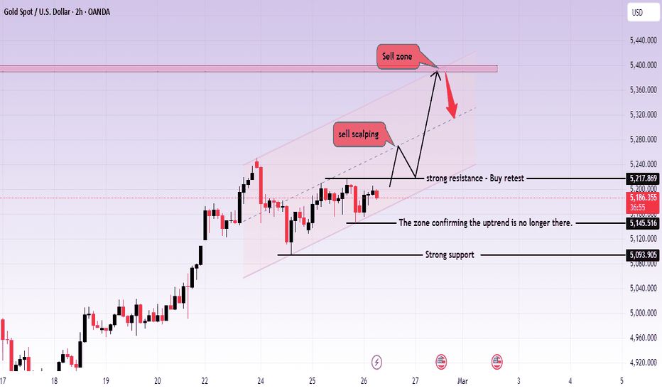
HAL 1 Week Time Frame 📌 Current approximate HAL price (latest available): around ₹3,950 – ₹4,010 per share (based on live NSE/BSE quotes).
📈 Weekly Resistance Levels — Upside (Targets)
These are zone prices where selling pressure might emerge:
R1 (Immediate): ~₹4,500 – ₹4,550
R2 (Medium): ~₹4,540 – ₹4,580
R3 (Extended): ~₹4,580 – ₹4,670
(A weekly close above ~₹4,580–₹4,600 may signal stronger bullish momentum.)
💡 Another pivot analysis shows similar weekly oppose points around ~₹4,276 – ₹4,383, and an upper resistance near ~₹4,471 for the current week’s range.
📉 Weekly Support Levels — Downside (Floors)
These are prices where buying interest might appear:
S1 (Immediate): ~₹4,420 – ₹4,380
S2 (Secondary): ~₹4,380 – ₹4,340
S3 (Lower): ~₹4,340 – ₹4,300
(Break below ~₹4,380 may open deeper correction toward ~₹4,300.)
Plus, for this specific week, analysts noted support zones around ~₹4,082 and ~₹3,994 – ₹3,888 if price pushes lower.
📌 Weekly Pivot Reference (Bias Indicator)
A pivot midpoint can help gauge bias:
Weekly Pivot: ~₹4,460 – ₹4,470
→ Above this pivot = slight bullish bias
→ Below pivot = neutral/bearish bias
📊 How Traders Often Use These Levels
Bullish scenario: If HAL sustains above first resistance zones (~₹4,500 +), the next targets could be nearer to ~₹4,550 – ₹4,670+.
Bearish scenario: A break below key support (~₹4,380) might see price testing deeper support near ~₹4,300 or weekly lower levels (~₹3,995 – ₹3,888).
Neutral/range: Price may oscillate within the support–resistance band if broader markets are sideways.
⚠️ These are technical price levels, not buy/sell recommendations — price can behave differently based on news (e.g., recent macro headlines affecting defence stocks). Always combine with risk management.  Long
Long
 Education

Education 
Education