Strategy

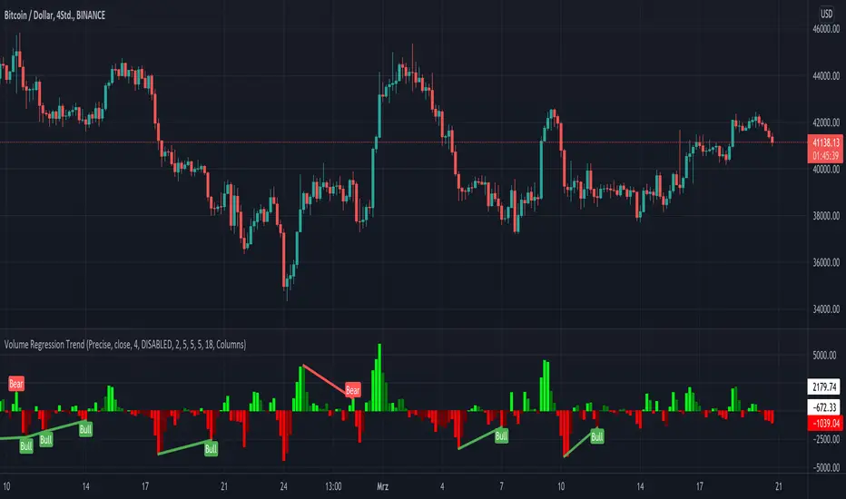
KINSKI Volume Regression TrendRegression trends are typically used to determine when a price is unusually far from its baseline. The script calculates the linear regression of volume and price to determine the trend direction and strength. This can be used to determine the volume support for upward/downward trends.
As a special feature, this indicator allows you to choose from three (as of 07/20/2021) templates with special presets.
The following templates are available:
"Precise" (Period: 4, Smoothing Factor Type: "DISABLED", Smoothing Factor Length = 1).
"Smooth" (Period: 4, Smoothing Factor Type: "RMA", Smoothing Factor Length = 2)
"Long Term (Period: 20, Smoothing Factor Type: "DISABLED", Smoothing Factor Length = 1)
In the selection for templates, the option "DISABLED" can also be selected. Then the user-defined settings selectable under it take effect. There are the following setting options.
"Length": Adjustable period
"Smoothing Factor: Type": Type of moving average
"Smoothing Factor: Length": Adjustable period
Other setting options are:
Color codes: The color codes are explained in the settings
Display types: "Columns", "Histogram", "Area", "Line", "Stepline"
Indicator

DAYOFWEEK performance1 -Objective
"What is the ''best'' day to trade .. Monday, Tuesday...."
This script aims to determine if there are different results depending on the day of the week.
The way it works is by dividing data by day of the week (Monday, Tuesday, Wednesday ... ) and perform calculations for each day of the week.
1 - Objective
2 - Features
3 - How to use (Examples)
4 - Inputs
5 - Limitations
6 - Notes
7 - Final Tooughs
2 - Features
AVG OPEN-CLOSE
Calculate de Percentage change from day open to close
Green % (O-C)
Percentage of days green (open to close)
Average Change
Absolute day change (O-C)
AVG PrevD. Close-Close
Percentage change from the previous day close to the day of the week close
(Example: Monday (C-C) = Friday Close to Monday close
Tuesday (C-C) = Monday C. to Tuesday C.
Green % (C1-C)
Percentage of days green (open to close)
AVG Volume
Day of the week Average Volume
Notes:
*Mon(Nº) - Nº = Number days is currently calculated
Example: Monday (12) calculation based on the last 12 Mondays. Note: Discrepancies in numbers example Monday (12) - Friday (11) depend on the initial/end date or the market was closed (Holidays).
3 - How to use (Examples)
For the following example, NASDAQ:AAPL from 1 Jan 21 to 1 Jul 21 the results are following.
The highest probability of a Close being higher than the Open is Monday with 52.17 % and the Lowest Tuesday with 38.46 %. Meaning that there's a higher chance (for NASDAQ:AAPL ) of closing at a higher value on Monday while the highest chance of closing is lower is Tuesday. With an average gain on Tuesday of 0.21%
Long - The best day to buy (long) at open (on average) is Monday with a 52.2% probability of closing higher
Short - The best day to sell (short) at open (on average) is Tuesday with a 38.5% probability of closing higher (better chance of closing lower)
Since the values change from ticker to ticker, there is a substantial change in the percentages and days of the week. For example let's compare the previous example ( NASDAQ:AAPL ) to NYSE:GM (same settings)
For the same period, there is a substantial difference where there is a 62.5% probability Friday to close higher than the open, while Tuesday there is only a 28% probability.
With an average gain of 0.59% on Friday and an average loss of -0.34%
Also, the size of the table (number of days ) depends if the ticker is traded or not on that day as an example COINBASE:BTCUSD
4 - Inputs
DATE RANGE
Initial Date - Date from which the script will start the calculation.
End Date - Date to which the script will calculate.
TABLE SETTINGS
Text Color - Color of the displayed text
Cell Color - Background color of table cells
Header Color - Color of the column and row names
Table Location - Change the position where the table is located.
Table Size - Changes text size and by consequence the size of the table
5 - LIMITATIONS
The code determines average values based on the stored data, therefore, the range (Initial data) is limited to the first bar time.
As a consequence the lower the timeframe the shorter the initial date can be and fewer weeks can be calculated. To warn about this limitation there's a warning text that appears in case the initial date exceeds the bar limit.
Example with initial date 1 Jan 2021 and end date 18 Jul 2021 in 5m and 10 m timeframe:
6 - Notes and Disclosers
The script can be moved around to a new pane if need. -> Object Tree > Right Click Script > Move To > New pane
The code has not been tested in higher subscriptions tiers that allow for more bars and as a consequence more data, but as far I can tell, it should work without problems and should be in fact better at lower timeframes since it allows more weeks.
The values displayed represent previous data and at no point is guaranteed future values
7 - Final Tooughs
This script was quite fun to work on since it analysis behavioral patterns (since from an abstract point a Tuesday is no different than a Thursday), but after analyzing multiple tickers there are some days that tend to close higher than the open.
PS: If you find any mistake ex: code/misspelling please comment.
Indicator

Indicator

Indicator

Grid Bot AutoThis script is an auto-adjusting grid bot simulator. This is an improved version of the original Grid Bot Simulator. The grid bot is best used for ranging/choppy markets. Prices are divided into grids, or trade zones, that will trigger signals each time a new zone is entered. During ranging markets, each transaction is followed by a “take profit.” As the market starts to trend, transactions are stacked (compare to DCA ), until the market consolidates. No signals are triggered above the Upper Limit or Below the Lower Limit. Unlike the previous version, the upper and lower limits are calculated automatically. Grid levels are determined by four factors: Smoothing, Laziness, Elasticity, and Grid Intervals.
Smoothing:
A moving average (or linear regression) is applied to each close price as a basis. Options for smoothing are Linear Regression, Simple Moving Average, Exponential Moving Average, Volume-Weighted Moving Average, Triple-Exponential Moving Average.
Laziness:
Laziness is the percentage change required to reach the next level. If laziness is 1.5, the price must move up or down by 1.5% before the grid will change. This concept is based on Alex Grover’s Efficient Trend Step. This allows the grids to be based on even price levels, as opposed to jagged moving averages.
Elasticity:
Elasticity is the degree of “stickiness” to the current price trend. If the smoothing line remains above (or below) the current grid center without reverting but still not enough to reach the next grid level, the grid line will start to curve toward the next grid level. Elasticity is added to (or subtracted from) the gridline by a factor of minimum system ticks for the current pair. Elasticity of zero will keep the gridlines horizontal. If elasticity is too high, the grid will distort.
Grid Intervals:
Grid intervals are the percentage of space between each grid.
Laziness = 4%, Elasticity = 0. Price must move at least 4% before reaching the next level. With zero elasticity, gridlines are straight.
Laziness = 5%, Elasticity = 100. For each bar at a new grid level, the grid will start “curve” toward the next price level (up if price is greater than the middle grid, down if less than middle grid). Elasticity is calculated by the user-inputted “Elasticity” multiplied by the minimum tick for the current pair (ELSTX = syminfo.mintick * iELSTX)
Try experimenting with different combinations of the Smoothing Length, Smoothing Type, Laziness, Elasticity, and Grid Intervals to find the optimum settings for each chart. Lower-priced pairs (e.g. XRP/ADA/DODGE) will require lower Elasticity. Also note that different exchanges may have different minimum tick values. For example, minimum tick for BITMEX:XBTUSD and BYBIT:BTCUSD is .5, but BINANCE:BTCUSDT and COINBASE:BTCUSD is .01.
s3.tradingview.com
DODGEUSDT, 5min. Laziness: 4%, Elasticity 2.5
Number of Grids: 2. Laziness: 3.75%. Elasticity: 150. Grid Interval 2%.
Settings Overview
Smoothing Length : Smoothing period
Smoothing Type : Linear Regression, Simple Moving Average, Exponential Moving Average, Volume-Weighted Moving Average, Triple-Exponential Moving Average
Laziness : Percentage required for price to move until it reaches the next level. If price does not reach the next level (up or down), the grid will remain the same as previous grid (because it’s lazy).
Elasticity : Amount of curvature toward the next grid, based on the current price trend. As elasticity increases, gridlines will curve up or down by a factor of the number of ticks since the last grid change.
Grid Interval : Percent between grid levels.
Number of Grids : Number of grids to show.
Cooldown : Number of bars to wait to prevent consecutive signals.
Grid Line Transparency : Lower transparencies brighten the gridlines; higher transparencies dim the gridlines. To hide the gridlines completely, enter 100.
Fill Transparency: Lower transparencies brighten the fill box; higher transparencies dim the fill box. To hide the fill box completely, enter 100.
Signal Size : Make signal triangles large or small.
Reset Buy/Sell Index When Grids Change : When a new grid is formed, resetting the index may prevent false signals (experimental)
Use Highs/Lows for Signals : If enabled, signals are triggered as soon as the price touches the next zone. If disabled, signals are triggered after bar closes. Enable this for “Once Per Bar alerts. Disable for “Once Per Bar Close” alerts.
Show Min Tick : If checked, syminfo.mintick is displayed in upper-righthand corner. Useful for estimating Laziness.
Reverse Fill Colors : Default fill for fill boxes is green after buy and red after sell. Check this box to reverse.
Note: The Grid Bot Simulator scripts are experimental and works in progress. Please feel free to comment or contact me if you have suggestions/complaints.
Indicator

Indicator
Indicator
Indicator

Indicator

Indicator

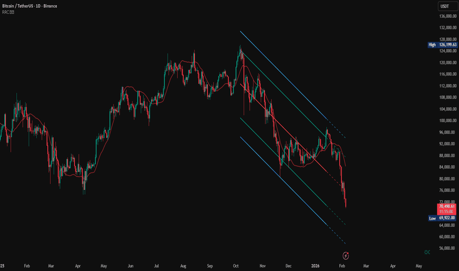
Raff Regression Channel by DGTRᴀꜰꜰ Rᴇɢʀᴇꜱꜱɪᴏɴ Cʜᴀɴɴᴇʟ (RRC)
This study aims to automate Raff Regression Channel drawing either based on ZigZag Indicator or optionally User Preference
The Raff Regression Channel , developed by Gilbert Raff, is based on a linear regression, which is the least-squares line-of-best-fit for a price series, with evenly spaced trend lines above and below . The width of the channel is set by determining the high or low that is the furthest from the linear regression.
Because the channel distance is based off the largest pullback or highest peak within a trend, for effectively drawing and using a Raff Regression Channel it is recommend/required that a Raff Regression Channel is applied to “mature” trends. Knowing this requirement, for better automated drawing results this study benefits from the Zig Zag Indicator, where the Zig Zag indicator is used to help identify price trends and changes in price trends. Option to manually adjust lengths for drawing a Raff Regression Channel is also made available.
Using a Raff Regression Channel
Once The Raff Regression Channel is drawn, covering an existing trend, Exᴛᴇɴꜱɪᴏɴ Lɪɴᴇꜱ are drawn to identify ᴛʜᴇ ꜱᴜᴘᴘᴏʀᴛ﹐ʀᴇꜱɪꜱᴛᴀɴᴄᴇ ᴏʀ ʀᴇᴠᴇʀꜱᴀʟ ᴘᴏɪɴᴛꜱ
The trend is up as long as prices rise within this channel. An uptrend may be reversing (not always, but likely) when price breaks below the channel extension . The trend is down as long as prices decline within the channel. Similarly, a downtrend may be reversing (not always, but likely) when price breaks above the channel extension . Moves outside the channel extensions can be indication of a reversal or can denote overbought or oversold conditions
For further details please refer to education post Raff Regression Channel
█ FEATURES
- AUTO or MANUALLY adjusted Raff Regression Channel and Channel Extentions drawing
- ALERTs, for Linear Regression Line, Raff Regression Upper and Lower Channel Extentions
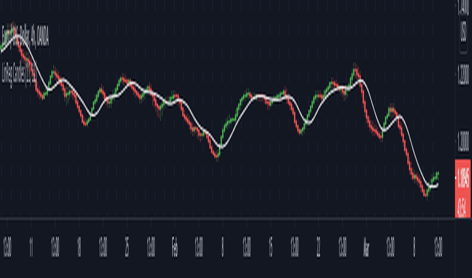
- LSMA , Least Squares Moving Average, in other words Linear Regression Curve
█ SETTINGS
Setting Loopback and Number of Bars are the most important part for The Raff Regression Channel, where ;
- Lookback, defines where the Raff Regression Channel is starting, it is recommended to set to a trend begining
- Number of Bars, defines how many bars to be assumed for calculation, or simply stated the end of the Raff Regression Channel drawing (not extentions but the main channel, extentions by default will be drawn till the last bar)
Setting of Loopback and Number of Bars is performed eigher automatically based on Zig Zag indicator or users may prefer to set them manually. If selected automatically then
- Deviation and Depth values of Zig Zag indicator are used for calculations (enabling visually plotting of ZigZag Lines will help to identify better visually the points), where ;
Deviation, is a multiplier that affects how much the price should deviate from the previous pivot in order for the bar to become a new pivot.
Depth, affects the minimum number of bars that will be taken into account when building
Short-term traders may wish to apply the channel to small waves of a trend so they can reduce the value of the Deviation and Depth
█ OTHER CHANNEL CONSEPTS
Linear Regression Channels, , what linear regression channels are? and linear regression channel/curve/slope study
Fibonacci Channels, how to apply fibonacci channels and automated fibonacci channels study
Andrews’ Pitchfork, how to apply pitchfork and automated pitchfork study
Special Thanks to @Kiss66000 for his kind suggestion, je vous remercie beaucoup @Kiss66000
Disclaimer :
Trading success is all about following your trading strategy and the indicators should fit within your trading strategy, and not to be traded upon solely
The script is for informational and educational purposes only. Use of the script does not constitute professional and/or financial advice. You alone have the sole responsibility of evaluating the script output and risks associated with the use of the script. In exchange for using the script, you agree not to hold dgtrd TradingView user liable for any possible claim for damages arising from any decision you make based on use of the script
Indicator
Indicator

Strategy

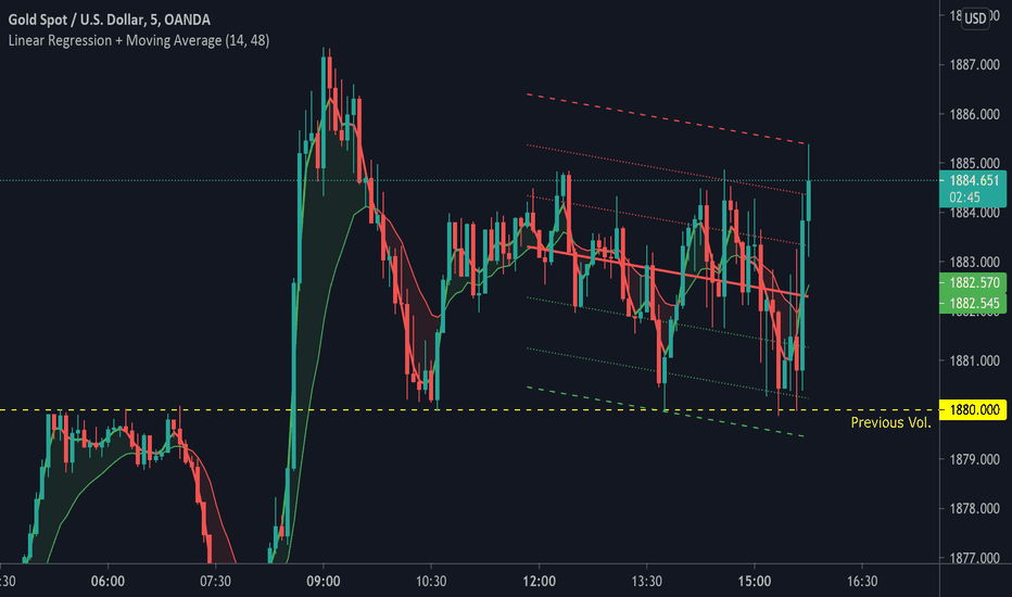
Linear Regression Channel / Curve / Slope by DGTTʜᴇ Lɪɴᴇᴀʀ Rᴇɢʀᴇꜱꜱɪᴏɴ Cʜᴀɴɴᴇʟꜱ
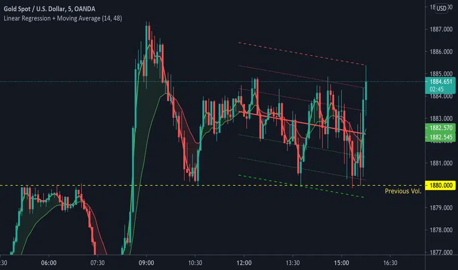
Linear Regression Channels are useful measure for technical and quantitative analysis in financial markets that help identifying trends and trend direction. The use of standard deviation gives traders ideas as to when prices are becoming overbought or oversold relative to the long term trend
The basis of a linear regression channel
Linear Regression Line – is a line drawn according to the least-squares statistical technique which produces a best-fit line that cuts through the middle of price action, a line that best fits all the data points of interest. The resulting fitted model can be used to summarize the data, to predict unobserved values from the same system. Linear Regression Line then present basis for the channel calculations
The linear regression channel
2. Upper Channel Line – A line that runs parallel to the Linear Regression Line and is usually one to two standard deviations above the Linear Regression Line.
3. Lower Channel Line – This line runs parallel to the Linear Regression Line and is usually one to two standard deviations below the Linear Regression Line.
Unlike Fibonacci Channels and Andrew’s Pitchfork, Linear Regression Channels are calculated using statistical methods, both for the regression line (as expressed above) and deviation channels. Upper and Lower channel lines are presenting the idea of bell curve method, also known as a normal distribution and are calculated using standard deviation function.
A standard deviation include 68% of the data points, two standard deviations include approximately 95% of the data points and any data point that appears outside two standard deviations is very rare.
It is often assumed that the data points will move back toward the average, or regress and channels would allow us to see when a security is overbought or oversold and ready to revert to the mean
please note : Over time, the price will move up and down, and the linear regression channel will experience changes as old prices fall off and new prices appear
█ Linear Regression Study Features
Linear Regression Channel
- Linear regression line as basis
- Customizable multiple channels based on Standard Deviation
- ALERTs for the channel levels
Linear Regression Curve
- Linear regression curve as basis
- Optional : Bands based on Standard Deviation or Volatility (ATR). Bands are applied with fixed levels 1, 2 and 3 times StdDev or ATR away from the curve
Linear Regression Slope
- Optional : Up/Down slope arrows for a used defined period
█ Volume / Volatility Add-Ons
High Volatile Bar Indication
Volume Spike Bar Indication
Volume Weighted Colored Bars
Indicator

Indicator

Indicator

Indicator

Indicator

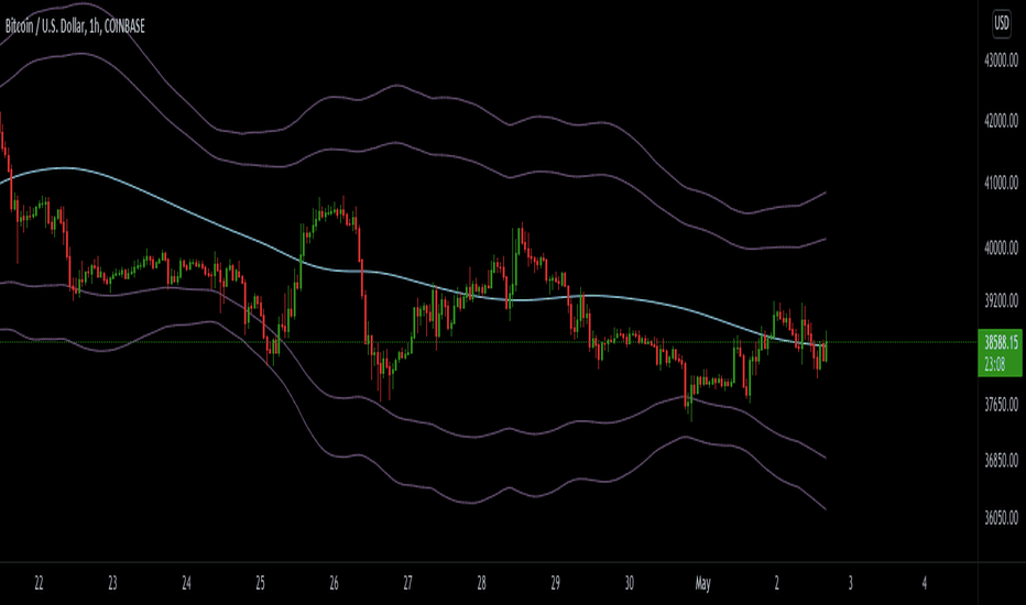
Robust Channel [tbiktag]Introducing the Robust Channel indicator.
This indicator is based on a remarkable property of robust statistics , namely, the resistance to the presence of data points that deviate significantly from the established trend (generally speaking, outliers ). Being outlier-resistant, the Robust Channel indicator “remembers” a pre-existing trend and thus exhibits a very peculiar "lag" in case of a sharp price change. This allows high-confidence identification of such price actions as a trend reversal, range break, pullback, etc.
In the case of trending and range-bound market conditions, the price remains within the channel most of the time, fluctuating around the central line.
Technical details
The central line is calculated using the repeated median slope algorithm. For each data point in a lookback window of a user-specified Length , this method calculates the median slope of the lines that connect that point to all other points inside the window. The overall median of these median slopes is then calculated and used as an estimate of the trend slope. The algorithm is very efficient as it uses an on-the-fly procedure to update the array containing the slopes (new data pushed - old data removed).
The outer line is then calculated as the central line plus the Length -period standard deviation of the price data multiplied by a user-defined Channel Width Factor . The inner line is defined analogously below the central line.
Usage
As a stand-alone indicator, the Robust Channel can be applied similarly to the Bollinger Bands and the Keltner Channel:
A close above the outer line can be interpreted as a bullish signal and a close below the inner line as a bearish signal.
Likewise, a return to the channel from below after a break may serve as a bullish signal, while a return from above may indicate bearish sentiment.
Robust Channel can be also used to confirm chart patterns such as double tops and double bottoms.
If you like this indicator, feel free to leave your feedback in the comments below!
Indicator

Indicator

Matrix Library (Linear Algebra, incl Multiple Linear Regression)What's this all about?
Ever since 1D arrays were added to Pine Script, many wonderful new opportunities have opened up. There has been a few implementations of matrices and matrix math (most notably by TradingView-user tbiktag in his recent Moving Regression script: ). However, so far, no comprehensive libraries for matrix math and linear algebra has been developed. This script aims to change that.
I'm not math expert, but I like learning new things, so I took it upon myself to relearn linear algebra these past few months, and create a matrix math library for Pine Script. The goal with the library was to make a comprehensive collection of functions that can be used to perform as many of the standard operations on matrices as possible, and to implement functions to solve systems of linear equations. The library implements matrices using arrays, and many standard functions to manipulate these matrices have been added as well.
The main purpose of the library is to give users the ability to solve systems of linear equations (useful for Multiple Linear Regression with K number of independent variables for example), but it can also be used to simulate 2D arrays for any purpose.
So how do I use this thing?
Personally, what I do with my private Pine Script libraries is I keep them stored as text-files in a Libraries folder, and I copy and paste them into my code when I need them. This library is quite large, so I have made sure to use brackets in comments to easily hide any part of the code. This helps with big libraries like this one.
The parts of this script that you need to copy are labeled "MathLib", "ArrayLib", and "MatrixLib". The matrix library is dependent on the functions from these other two libraries, but they are stripped down to only include the functions used by the MatrixLib library.
When you have the code in your script (pasted somewhere below the "study()" call), you can create a matrix by calling one of the constructor functions. All functions in this library start with "matrix_", and all constructors start with either "create" or "copy". I suggest you read through the code though. The functions have very descriptive names, and a short description of what each function does is included in a header comment directly above it. The functions generally come in the following order:
Constructors: These are used to create matrices (empy with no rows or columns, set shape filled with 0s, from a time series or an array, and so on).
Getters and setters: These are used to get data from a matrix (like the value of an element or a full row or column).
Matrix manipulations: These functions manipulate the matrix in some way (for example, functions to append columns or rows to a matrix).
Matrix operations: These are the matrix operations. They include things like basic math operations for two indices, to transposing a matrix.
Decompositions and solvers: Next up are functions to solve systems of linear equations. These include LU and QR decomposition and solvers, and functions for calculating the pseudo-inverse or inverse of a matrix.
Multiple Linear Regression: Lastly, we find an implementation of a multiple linear regression, including all the standard statistics one can expect to find in most statistical software packages.
Are there any working examples of how to use the library?
Yes, at the very end of the script, there is an example that plots the predictions from a multiple linear regression with two independent (explanatory) X variables, regressing the chart data (the Y variable) on these X variables. You can look at this code to see a real-world example of how to use the code in this library.
Are there any limitations?
There are no hard limiations, but the matrices uses arrays, so the number of elements can never exceed the number of elements supported by Pine Script (minus 2, since two elements are used internally by the library to store row and column count). Some of the operations do use a lot of resources though, and as a result, some things can not be done without timing out. This can vary from time to time as well, as this is primarily dependent on the available resources from the Pine Script servers. For instance, the multiple linear regression cannot be used with a lookback window above 10 or 12 most of the time, if the statistics are reported. If no statistics are reported (and therefore not calculated), the lookback window can usually be extended to around 60-80 bars before the servers time out the execution.
Hopefully the dev-team at TradingView sees this script and find ways to implement this functionality diretly into Pine Script, as that would speed up many of the operations and make things like MLR (multiple linear regression) possible on a bigger lookback window.
Some parting words
This library has taken a few months to write, and I have taken all the steps I can think of to test it for bugs. Some may have slipped through anyway, so please let me know if you find any, and I'll try my best to fix them when I have time to do so. This library is intended to help the community. Therefore, I am releasing the library as open source, in the hopes that people may improving on it, or using it in their own work. If you do make something cool with this, or if you find ways to improve the code, please let me know in the comments.
Indicator

Indicator