ChartRage - ELMAELMA - Exponential Logarithmic Moving Average
This is a new kind of moving average that is using exponential normalization of a logarithmic formula. The exponential function is used to average the weight on the moving average while the logarithmic function is used to calculate the overall price effect.
Features and Settings:
◻️ Following rate of change instead of absolute levels
◻️ Choose input source of the data
◻️ Real time signals through price interaction
◻️ Change ELMA length
◻️ Change the exponential decay rate
◻️ Customize base color and signal color
Equation of the ELMA:
This formula calculates a weighted average of the logarithm of prices, where more recent prices have a higher weight. The result is then exponentiated to return the ELMA value. This approach emphasizes the relative changes in price, making the ELMA sensitive to the % rate of change rather than absolute price levels. The decay rate can be adjusted in the settings.
Comparison EMA vs ELMA:
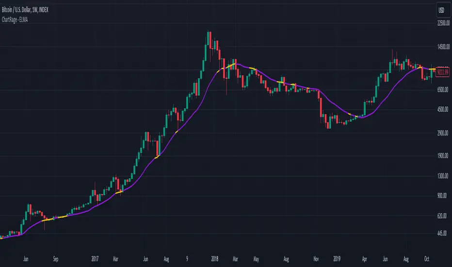
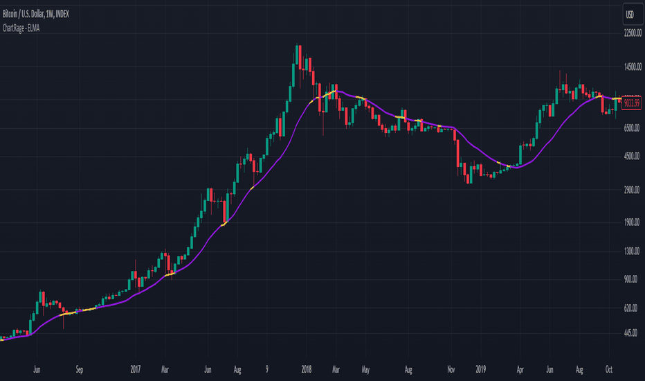
In this image we see the differences to the Exponential Moving Average.
Price Interaction and earlier Signals:
In this image we have added the bars, so we can see that the ELMA provides different signals of resistance and support zones and highlights them, by changing to the color yellow, when prices interact with the ELMA.
Strategy by trading Support and Resistance Zones:
The ELMA helps to evaluate trends and find entry points in bullish market conditions, and exit points in bearish conditions. When prices drop below the ELMA in a bull market, it is considered a buying signal. Conversely, in a bear market, it serves as an exit signal when prices trade above the ELMA.
Volatile Markets:
The ELMA works on all timeframes and markets. In this example we used the default value for Bitcoin. The ELMA clearly shows support and resistance zones. Depending on the asset, the length and the decay rate should be adjusted to provide the best results.
Real Time Signals:
Signals occur not after a candle closes but when price interacts with the ELMA level, providing real time signals by shifting color. (default = yellow)
Disclaimer* All analyses, charts, scripts, strategies, ideas, or indicators developed by us are provided for informational and educational purposes only. We do not guarantee any future results based on the use of these tools or past data. Users should trade at their own risk.
This work is licensed under Attribution-NonCommercial-ShareAlike 4.0 International
creativecommons.org Indicator
Adaptive Trend Finder (log)In the dynamic landscape of financial markets, the Adaptive Trend Finder (log) stands out as an example of precision and professionalism. This advanced tool, equipped with a unique feature, offers traders a sophisticated approach to market trend analysis: the choice between automatic detection of the long-term or short-term trend channel.
Key Features:
1. Choice Between Long-Term or Short-Term Trend Channel Detection: Positioned first, this distinctive feature of the Adaptive Trend Finder (log) allows traders to customize their analysis by choosing between the automatic detection of the long-term or short-term trend channel. This increased flexibility adapts to individual trading preferences and changing market conditions.
2. Autonomous Trend Channel Detection: Leveraging the robust statistical measure of the Pearson coefficient, the Adaptive Trend Finder (log) excels in autonomously locating the optimal trend channel. This data-driven approach ensures objective trend analysis, reducing subjective biases, and enhancing overall precision.
3. Precision of Logarithmic Scale: A distinctive characteristic of our indicator is its strategic use of the logarithmic scale for regression channels. This approach enables nuanced analysis of linear regression channels, capturing the subtleties of trends while accommodating variations in the amplitude of price movements.
4. Length and Strength Visualization: Traders gain a comprehensive view of the selected trend channel, with the revelation of its length and quantification of trend strength. These dual pieces of information empower traders to make informed decisions, providing insights into both the direction and intensity of the prevailing trend.
In the demanding universe of financial markets, the Adaptive Trend Finder (log) asserts itself as an essential tool for traders, offering an unparalleled combination of precision, professionalism, and customization. Highlighting the choice between automatic detection of the long-term or short-term trend channel in the first position, this indicator uniquely caters to the specific needs of each trader, ensuring informed decision-making in an ever-evolving financial environment. Indicator

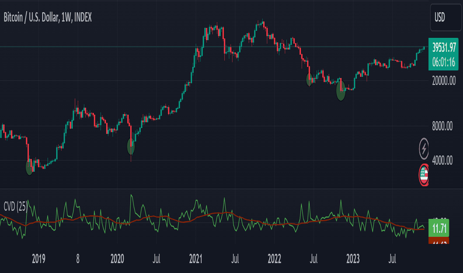
Logarithmic CVD [IkkeOmar]The LCVD is another Mean-Reversion Indicator. it doesn't detect trends and does not give a signal per se. However the logarithmic transformation is made to visualize the direction of the trend for the volume. This allows you to see if money is flowing in or out of an asset.
What it does is tell you if we have a flashcrash based on the difference in volume.
Think of this indicator like a form of a volatility index.
Smoothing input:
The only input is an input for the smoothing length of the logDelta.
Volume Calculation:
// @IkkeOmar
//@version=5
indicator('Logarithmic CVD', shorttitle='CVD', overlay=false)
smooth = input.int(defval = 25, title = "Smoothing Distance")
// Calculate buying and selling volume
askVolume = volume * (close > open ? 1 : 0) // Assuming higher close than open indicates buying
bidVolume = volume * (close < open ? 1 : 0) // Assuming lower close than open indicates selling
// Delta is the difference between buying and selling volume
delta = askVolume - bidVolume
// Apply logarithmic transformation to delta
// Adding a check to ensure delta is not zero as log(0) is undefined
logDelta = delta > 0 ? math.log(math.abs(delta)) * math.sign(delta) : - math.log(math.abs(delta)) * math.sign(delta)
// use the the ta lib for calculating the sma of the logDelta
smoothLogDelta = ta.sma(logDelta, smooth)
// Create candlestick plot
plot(logDelta, color= color.green, title='Logarithmic CVD')
plot(smoothLogDelta, color= color.rgb(145, 37, 1), title='Smooth CVD')
These lines calculate the buying and selling volumes. askVolume is calculated as the total volume when the closing price is higher than the opening price, assuming this indicates buying pressure. bidVolume is calculated as the total volume when the closing price is lower than the opening price, assuming selling pressure.
The Delta is simply the difference between buying and selling volumes.
Logarithmic Transformation:
logDelta = delta > 0 ? math.log(math.abs(delta)) * math.sign(delta) : - math.log(math.abs(delta)) * math.sign(delta)
Applies a logarithmic transformation to delta. The math.log function is used to calculate the natural logarithm of the absolute value of delta. The sign of delta is preserved to differentiate between positive and negative values. This transformation helps in scaling the delta values, especially useful when dealing with large numbers.
This script essentially provides a visual representation of the buying and selling pressures in a market, transformed logarithmically for better scaling and smoothed for trend analysis.
Hope it makes sense!
Stay safe everyone!
Don't hesitate to ask any questions if you have any!
Indicator
Logarithmic Volatility Direction Index [IkkeOmar]The LVDI is a Mean-Reversion Indicator. it doesn't detect trends and does not give a signal per se.
What it does is tell you if we have a flashcrash based on the price action and volume that is available. It is not always easy to see with the naked eye, so this indicator can help you DCA into an asset in a smarter way, if you couple it with other trend systems.
Think of this indicator like a form of a volatility index.
Inputs:
len and lenWMA are integers representing different lengths for calculations, and src is the data source
Keep in mind that "Length" is the lookback for the WMA, and the Length smooting is the lookback for the SMA of the "volume_weighted".
WMA Calculation
wma_basic = math.log10(ta.wma(src, len))
This calculates the logarithm (base 10) of the Weighted Moving Average (WMA) of the source data over len periods. WMA is a type of moving average giving more importance to recent data. The reason I use log10, is to make it transformative over a longer timeframe. This makes it easier to see the growth direction. I like to use this for crypto, since there is asymetric upside.
Volume Filter:
average_volume = ta.sma(volume, lenWMA)
volume_weighted = math.log10(wma_basic * (volume / math.log10(average_volume)))
Here, the script first calculates the Simple Moving Average (SMA) of the trading volume over lenWMA periods. Then, it computes a volume-weighted value of the WMA, adjusted by the logarithmic ratio of current volume to average volume.
Distance and Score Calculation:
distance = math.log10(src) - math.log10(volume_weighted)
score = math.sign(distance) * math.pow(math.abs(distance), 2)
The script calculates the logarithmic difference between the source data and the volume-weighted WMA. The score is determined by the sign of this distance multiplied by its square. This potentially amplifies the impact of larger distances.
Plotting:
plot(volume_weighted, title="Volume Weighted WMA", color=color.blue, linewidth = 2)
plot(ta.sma(volume_weighted, lenWMA), title="Volume Weighted WMA", color=color.rgb(189, 160, 0))
Mathematical concepts
Weighted Moving Average (WMA):
WMA is a moving average that assigns more weight to recent data points. The idea is that recent prices are more relevant to the current trend than older prices.
Logarithms:
The use of log10 (logarithm base 10) is interesting. Logarithms help in normalizing data and can make certain patterns more visible, especially when dealing with exponential growth or decay.
Volume Weighting:
Multiplying the WMA by the ratio of current volume to average volume (both logarithmic) integrates volume into the analysis. High trading volume can signify stronger market interest and can thus validate price movements.
Distance and Score:
The distance measures how far the current price is from the volume-weighted WMA on a logarithmic scale. The score squares this distance, potentially highlighting large divergences.
Case example
In the case above (which is a low timeframe that shouldn't be your main system) we see the blue line going up before going below the moving average line (orange). This indicates a local bottom zone. Does that mean that we wont go lower? No! What you can do is calculate a zone range.
We have an average line, you can get that from the POC with the VRVP.
Then you take the low and high of that zone and take the average:
(3.17% + 2.33%) / 2 = 2.75%
This means that we expect that the price can fall an additional 2.75%! Low and behold. When you check the same chart as above:
Hope it makes sense!
Stay safe everyone!
Don't hesitate to ask any questions if you have any! Indicator

Nadaraya-Watson Envelope Strategy (Non-Repainting) Log ScaleIn the diverse world of trading strategies, the Nadaraya-Watson Envelope Strategy offers a different approach. Grounded in mathematical analysis, this strategy utilizes the Nadaraya-Watson kernel regression, a method traditionally employed for interpreting complex data patterns.
At the core of this strategy lies the concept of 'envelopes', which are essentially dynamic volatility bands formed around the price based on a custom Average True Range (ATR). These envelopes help provide guidance on potential market entry and exit points. The strategy suggests considering a buy when the price crosses the lower envelope and a sell when it crosses the upper envelope.
One distinctive characteristic of the Nadaraya-Watson Envelope Strategy is its use of a logarithmic scale, as opposed to a linear scale. The logarithmic scale can be advantageous when dealing with larger timeframes and assets with wide-ranging price movements.
The strategy is implemented using Pine Script v5, and includes several adjustable parameters such as the lookback window, relative weighting, and the regression start point, providing a level of flexibility.
However, it's important to maintain a balanced view. While the use of mathematical models like the Nadaraya-Watson kernel regression may provide insightful data analysis, no strategy can guarantee success. Thorough backtesting, understanding the mathematical principles involved, and sound risk management are always essential when applying any trading strategy.
The Nadaraya-Watson Envelope Strategy thus offers another tool for traders to consider. As with all strategies, its effectiveness will largely depend on the trader's understanding, application, and the specific market conditions. Strategy

Adaptive Price Channel (log scale)The field of technical analysis is consistently expanding, with numerous indicators used for market forecasting. Amongst them, a novel indicator dubbed the Adaptive Price Channel (log scale), inspired by the renowned Nadaraya-Watson Envelope (LuxAlgo) from LuxAlgo, is gaining traction for its distinctive features and versatility. Unlike its predecessor, the Adaptive Price Channel (log scale) is applicable on a logarithmic scale, thereby allowing it to be utilized on both smaller and larger timeframes.
1. Key Features
The Adaptive Price Channel (log scale) is founded on the trading view Pinescript language, version 5, with its primary aim to maximize the versatility and scalability of trading indicators. It allows traders to adapt it according to their preferred timeframe, thereby making it applicable for a wide range of trading strategies.
Its bandwidth can be adjusted through the input parameters, offering traders the flexibility to manipulate the indicator according to their strategic requirements. Furthermore, it provides an option for repainting smoothing. This option enables users to control the repainting effect in which the historical output of the indicator may change over time. When disabled, the indicator provides the endpoints of the calculations, ensuring consistency in historical values.
Moreover, the Adaptive Price Channel (log scale) allows for color customization, thereby improving visibility and user-friendliness. The colors of the indicator's upward and downward directions can be changed according to the user's preference.
2. Working Mechanism
The Adaptive Price Channel (log scale) uses the logarithm of the source, which is typically the closing price of a trading instrument. It leverages a Gaussian function that exponentially decreases the further the price moves away from the mean, accounting for both positive and negative values. The bandwidth of the Gaussian function can be adjusted to adapt to different market conditions.
Additionally, the Adaptive Price Channel (log scale) features an array of 500 lines for each bar, which helps in defining the boundaries or envelope for price movements. The calculations are executed using the Nadaraya-Watson estimator, which uses kernel regression for non-parametric analysis.
The calculated values for the upper and lower bounds of the envelope are then converted back from the logarithmic scale using the exponential function. This calculation process continues for each bar until the last bar in the data set.
To ensure optimal performance, the Adaptive Price Channel (log scale) uses dynamic repainting. If the repainting mode is enabled, it adjusts the smoothing of the indicator for the entire historical data, making the results more accurate.
3. Visualization and Alerts
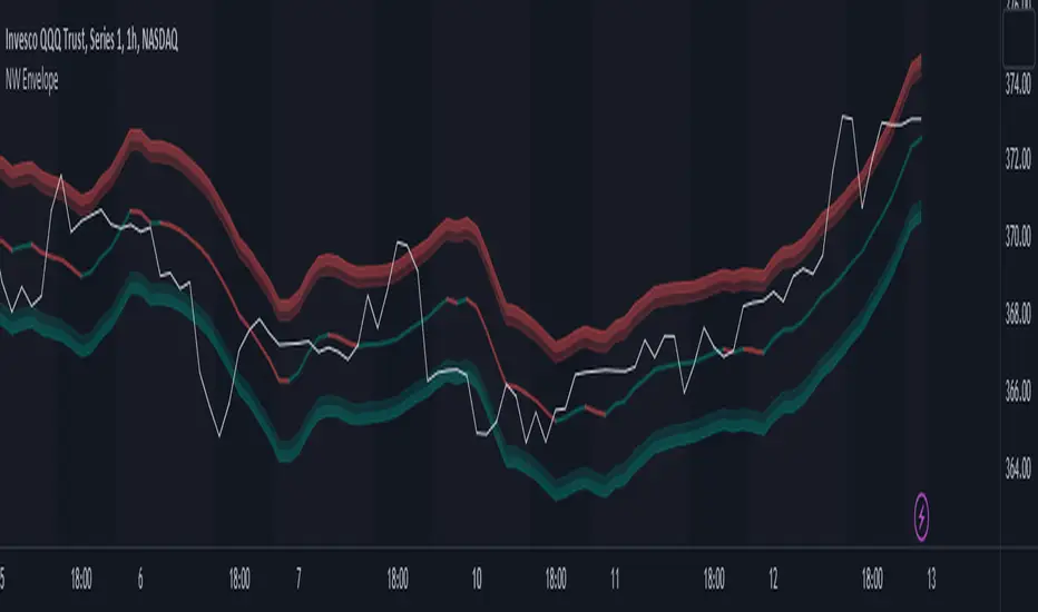
The Adaptive Price Channel (log scale) offers an array of visual aids, including labels and plots. The upper and lower bounds of the envelope are plotted, and the indicator triggers labels at points where the closing price crosses these boundaries. These labels serve as alerts for potential trading opportunities.
4. Conclusion
The Adaptive Price Channel (log scale) is an innovative and adaptable trading indicator, drawing inspiration from its predecessor but introducing unique features to increase its versatility. By providing a repainting option, it ensures consistent historical values, thereby enhancing the reliability of the indicator. Furthermore, the capability to operate on a logarithmic scale broadens its usability for different timeframes. The Adaptive Price Channel (log scale) is a powerful tool for any trader, facilitating a better understanding of market dynamics, and enabling more informed decision-making. Indicator

Nadaraya-Watson Envelope (Non-Repainting) Logarithmic ScaleIn the fast-paced world of trading, having a reliable and accurate indicator can make all the difference. Enter the Nadaraya-Watson Envelope Indicator, a cutting-edge tool designed to provide traders with valuable insights into market trends and potential price movements. In this article, we'll explore the advantages of this non-repainting indicator and how it can empower traders to make informed decisions with confidence.
Accurate Price Analysis:
The Nadaraya-Watson Envelope Indicator operates in a logarithmic scale, allowing for more accurate price analysis. By considering the logarithmic nature of price movements, this indicator captures the subtle nuances of market dynamics, providing a comprehensive view of price action. Traders can leverage this advantage to identify key support and resistance levels, spot potential breakouts, and anticipate trend reversals.
Non-Repainting Reliability:
One of the most significant advantages of the Nadaraya-Watson Envelope Indicator is its non-repainting nature. Repainting indicators can mislead traders by changing historical signals, making it difficult to evaluate past performance accurately. With the non-repainting characteristic of this indicator, traders can have confidence in the reliability and consistency of the signals generated, ensuring more accurate backtesting and decision-making.
Customizable Parameters:
Every trader has unique preferences and trading styles. The Nadaraya-Watson Envelope Indicator offers a range of customizable parameters, allowing traders to fine-tune the indicator to their specific needs. From adjusting the lookback window and relative weighting to defining the start of regression, traders have the flexibility to adapt the indicator to different timeframes and trading strategies, enhancing its effectiveness and versatility.
Envelope Bounds and Estimation:
The Nadaraya-Watson Envelope Indicator calculates upper and lower bounds based on the Average True Range (ATR) and specified factors. These envelope bounds act as dynamic support and resistance levels, providing traders with valuable reference points for potential price targets and stop-loss levels. Additionally, the indicator generates an estimation plot, visually representing the projected price movement, enabling traders to anticipate market trends and make well-informed trading decisions.
Visual Clarity with Plots and Fills:
Clear visualization is crucial for effective technical analysis. The Nadaraya-Watson Envelope Indicator offers plots and fills to enhance visual clarity and ease of interpretation. The upper and lower boundaries are plotted, along with the estimation line, allowing traders to quickly assess price trends and volatility. Fills between the boundaries provide a visual representation of different price regions, aiding in identifying potential trading opportunities and risk management.
Conclusion:
The Nadaraya-Watson Envelope Indicator is a powerful tool for traders seeking accurate and reliable insights into market trends and price movements. With its logarithmic scale, non-repainting nature, customizable parameters, and visual clarity, this indicator equips traders with a competitive edge in the financial markets. By harnessing the advantages offered by the Nadaraya-Watson Envelope Indicator, traders can navigate the complexities of trading with confidence and precision. Unlock the potential of this advanced indicator and elevate your trading strategy to new heights. Indicator

Indicator

Indicator

Indicator

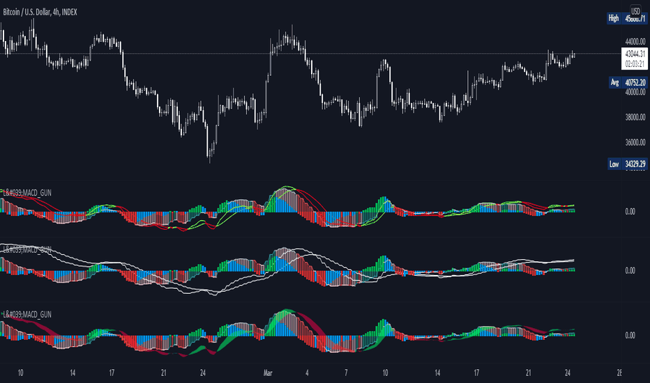
L'MACD GUNHi all!
I would like to present you my universal MACD module.
In addition to the standard functions I have added several improvements:
Source Selection.
In addition to the standard calculation of the moving average "EMA", in the parameter "MA Type" I have added 52 more methods for calculating the MA! :
ADXMA, AHMA, ALF, ALMA, ARI, ARSI, BlackFilter, CTI, DoubleEma, DTA, DWMA, EEO, EHMA, ELA, EMARSI, EREA, HEMA, hma, HWMA, JAMA, KA, KAMA, LSMA, LWMA, McGinley_2, MNMA, PAW, REMA, rma, RMF, RMTA, RWMA, sma, SMMA, SuperSmooth, THMA, TilsonT3, TMA, TRAMA, TripleEma, TSF, VAMA, VAR, VHMA, VIDYA, VVMA, vwma, WCD, wma, WWMA, ZEMA, ZLMA !
Additional histogram and lines from the higher timeframe. With the parameter "Multiple of TF" you can specify on which timeframe the standard histogram should be zoomed.
The Zoom function allows increasing or decreasing the size of the histogram. (It does not affect the calculations in any way, it is only used for visualization purposes.)
How to use it?
I recommend using it as a standard MACD. You can test different types of moving averages thanks to my modules and choose the one you find most suitable.
Tips:
The script is slightly heavy and may take a little longer to load than usual.
All MA types are in alphabetical order and tied to numbers.
Next to the "MA Type" parameter there is a hint which method of calculating MA corresponds to the figure. The default is 15. In the hint 15 = EMA. This is the standard method of calculating the MAСD.
To select the MA more quickly. You can switch them with the mouse wheel or the arrows on the keyboard.
I use the standard parameters prescribed in the script.
The code is calibrated for any TF and displays as correctly as possible. Can be used on any type of chart. Indicator
Indicator
Indicator

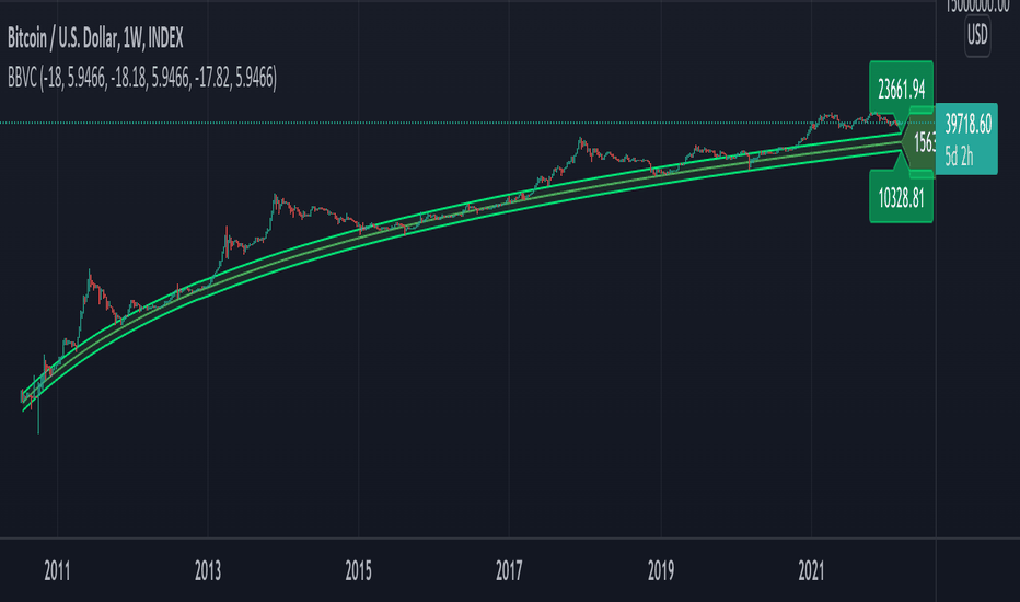
Logarithmic Bollinger BandsLogarithmic Bollinger Bands
Published by Eric Thies on January 14, 2022
Summary
In this script I have taken the standard Bollinger band pinescript and made efforts to eliminate the behavior experienced in periods of high volatility in which we see the bands disappear completely off the chart by adding exponential plotting and logarithmic sourcing to the tool.
This tool will also show periods of Bearish and Bullish Expansion for users to see when volatility is running high in the market.
More On Bollinger Bands
Bollinger Bands consist of a center line representing the moving average of a security’s price over a certain period, and two additional parallel lines (called the upper and lower trading bands) one of which is just the moving average plus k-times the standard deviation over the selected time frame, and the other being the moving average minus k-times the standard deviation over that same timeframe. This technique has been developed in the 1980’s by John Bollinger, who lately registered the terms “Bollinger Bands” as a U.S. trademark in 2011. Technical analysts typically use 20 periods and k = 2 as default settings to build Bollinger Bands, while they can choose a simple or exponential moving average. Bollinger Bands provide a relative definition of high and low prices of a security. When the security is trading within the upper band, the price is considered high, while it is considered low when the security is trading within the lower band.
There is no general consensus on the use of Bollinger Bands among traders. Some traders see a buy signal when the price hits the lower Bollinger Band and close their position when the price hits the moving average. Some others buy when the price crosses over the upper band and sell when the price crosses below the lower band. We can see here two opposing interpretations based on different rationales, depending whether we are in a reversal or continuation pattern. Another interesting feature of the Bollinger Bands is that they give an indication of the volatility levels; a widening gap between the upper and lower bands indicates an increasing volatility, while a narrowing band indicates a decreasing volatility. Moreover, when the bands have an almost flat slope (parallel to the x-axis) the price will generally oscillate between the bands as if trading through a channel.
// © 2022 KINGTHIES THIS SOURCE CODE IS SUBJECT TO TERMS OF MOZILLA PUBLIC LICENSE 2.0 (MOZILLA.ORG/MPL/2.0)
//@version=5
//## !<---------------- © KINGTHIES --------------------->
indicator('Logarithmic Bollinger Bands (kingthies)',shorttitle='LogBands_KT',overlay=true)
// { BBANDS
src = math.log(input(close,title="Source"))
lenX = input(20,title='lenX')
highlights = input(false,title="Highlight Bear and Bull Expansions?")
mult = 2
bbandBasis = ta.sma(src,lenX)
dev = 2 * ta.stdev(src, 20)
upperBB = bbandBasis + dev
lowerBB = bbandBasis - dev
bbw = (upperBB-lowerBB)/bbandBasis
bbr = (src - lowerBB)/(upperBB - lowerBB)
// }
// { BBAND EXPANSIONS
bullExp= ta.rising(upperBB,1) and ta.falling(lowerBB,1) and ta.rising(bbandBasis,1) and ta.rising(bbw,1) and ta.rising(bbr,1)
bearExp= ta.rising(upperBB,1) and ta.falling(lowerBB,1) and ta.falling(bbandBasis,1) and ta.rising(bbw,1) and ta.falling(bbr,1)
// }
// { COLORS
greenBG = color.rgb(9,121,105,75), redBG = color.rgb(136,8,8,75)
bullCol = highlights and bullExp ? greenBG : na, bearCol = highlights and bearExp ? redBG : na
// }
// { INDICATOR PLOTTING
lowBB=plot(math.exp(lowerBB),title='Low Band',color=color.aqua),plot(math.exp(bbandBasis),title='BBand Basis',color=color.red),
highBB=plot(math.exp(upperBB),title='High Band',color=color.aqua),fill(lowBB,highBB,title='Band Fill Color',color=color.rgb(0,128,128,75))
bgcolor(bullCol,title='Bullish Expansion Highlights'),bgcolor(bearCol,title='Bearish Expansion Highlights')
// }
Indicator

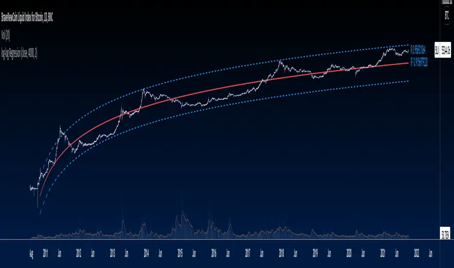
Universal logarithmic growth curves, with support and resistanceLogarithmic regression is used to model data where growth or decay accelerates rapidly at first and then slows over time. This model is for the long term series data (such as 10 years time span).
The user can consider entering the market when the price below 25% or 5% confidence and consider take profit when the price goes above 75% or 95% confidence line.
This script is:
- Designed to be usable in all tickers. (not only for bitcoin now!)
- Logarithmic regression and shows support-resistance level
- Shape of lines are all linear adjustable
- Height difference of levels and zones are customizable
- Support and resistance levels are highlighted
Input panel:
- Steps of drawing: Won't change it unless there are display problems.
- Resistance, support, other level color: self-explanatory.
- Stdev multipliers: A constant variable to adjust regression boundaries.
- Fib level N: Base on the relative position of top line and base line. If you don't want all fib levels, you might set all fib levels = 0.5.
- Linear lift up: vertically lift up the whole set of lines. By linear multiplication.
- Curvature constant: It is the base value of the exponential transform before converting it back to the chart and plotting it. A bigger base value will make a more upward curvy line.
FAQ:
Q: How to use it?
A: Click "Fx" in your chart then search this script to get it into your chart. Then right click the price axis, then select "Logarithmic" scale to show the curves probably.
Q: Why release this script?
A: - This script is intended to to fix the current issues of bitcoins growth curve script, and to provide a better version of the logarithmic curve, which is not only for bitcoin , but for all kinds of tickers.
- In the public library there is a hardcoded logarithmic growth curve by @quantadelic . But unfortunately that curve was hardcoded by his manual inputs, which makes the curve stop updating its value since 2019 the date he publish that code. Many users of that script love using it but they realize it was stop updating, many users out there based on @quantadelic version of "bitcoin logarithmic growth curves" and they tried their best to update the coordinates with their own hardcode input values. Eventually, a lot of redundant hardcoded "Bitcoin growth curve" scripts was born in the public library. Which is not a good thing.
Q: What about looking at the regression result with a log scale price axis?
A: You can use this script that I published in a year ago. This script display the result in a log scale price axis.
Indicator

Indicator

LineGetPriceOnLogScaleLibrary "LineGetPriceOnLogScale"
This library provides a way to calculate the y-coordinate of a line on a specified bar when the chart scale is Log.
The built-in `line.get_price()` function only works with linear scale and gives incorrect results when the chart is in Log scale.
The library only works with `bar_index` values and `xloc.bar_index`-based lines, `time`-based lines will cause errors to appear.
coordGetPriceLog(x1, y1, x2, y2, xi) Calculates the y-coordinate on the specified bar on the logarithmic scale.
Only coordinates based on bar index are applicable, bar time will throw an error.
Parameters:
x1 : First X coordinate of a line, index of the bar where the line starts.
y1 : First Y coordinate of a line, price on the price scale.
x2 : Second X coordinate of a line, index of the bar where the line ends.
y2 : Second Y coordinate of a line, price on the price scale.
xi : Index of the bar for which the price should be calculated.
Returns: Price of the line on the bar specified in `xi`, on the logarithmic scale.
lineGetPriceLog(_line, xi) Calculates the y-coordinate on the specified bar for the logarithmic scale. Takes a line.
Only lines drawn based on `xloc.bar_index` are applicable, `xloc.bar_time` will throw and error.
Parameters:
_line : The line for which the price is calculated.
xi : Index of the bar for which the bar should calculate the price.
Returns: Price of the line on the bar specified in `xi`, on the logarithmic scale. Library

Indicator

Auto Phivots S/R [DM]Greetings colleagues
Today I share the classic pivot points indicator
Added options:
Standard levels
Fibonacci levels "up to 261'8"
Logarithmic scale option
//Pivot Points Standard
//Pivot Points Standard — is a technical indicator that is used to determine the levels
//at which price may face support or resistance. The Pivot Points indicator consists of
//a pivot point (PP) level and several support (S) and resistance (R) levels.
//
//Calculation
//PP, resistance and support values are calculated in different ways, depending on
//the type of the indicator, specified by the Type field in indicator inputs. To
//calculate PP and support/resistance levels, the values OPENcurr, OPENprev, HIGHprev,
//LOWprev, CLOSEprev are used, which are the values of the current open and previous
//open, high, low and close, respectively, on the indicator resolution. The indicator
//resolution is set by the input of the Pivots Timeframe. If the Pivots Timeframe is set
//to AUTO (the default value), then the increased resolution is determined by the
//following algorithm:
//
//for intraday resolutions up to and including 15 min, DAY (1D) is used
//for intraday resolutions more than 15 min, WEEK (1W) is used
//for daily resolutions MONTH is used (1M)
//for weekly and monthly resolutions, 12-MONTH (12M) is used
Indicator

Indicator

Indicator

Indicator

Indicator