
After RSI produced nothing and the Turn of the Month effect produced something, the obvious next question was VWAP. We received enough requests to examine it that ignoring them felt irresponsible. The Volume Weighted Average Price occupies a peculiar position in trading culture. Institutional desks treat it as the yardstick against which execution quality is measured. Retail traders treat it as a crystal ball. One side built a trillion-dollar execution infrastructure around it. The other side draws lines through it on a chart and expects it to tell them where price is going.
We tested this properly. Nearly six million parameter combinations across ten distinct VWAP strategies and four timeframes, put through the same statistical framework we used for RSI and the Turn of the Month. The results surprised us. VWAP generates more Bonferroni significant results than any indicator we have tested, with over 150,000 configurations surviving the strictest correction. Mean reversion short signals produce an average edge of 0.89 percentage points, roughly six times typical transaction costs. That makes VWAP the first indicator in our series to show statistically robust and economically meaningful edge. The catch: this edge concentrates in a single strategy type. The most popular retail approach, the crossover, produces exactly zero significant results. Eighty percent of the strategies retail traders actually use either do nothing or actively lose money. VWAP has real predictive value, but almost nobody is using it correctly.
Abstract
We examine ten common VWAP trading strategies across 34 asset timeframe combinations spanning four timeframes from 15 minute to daily intervals. Testing 5,833,435 parameter configurations including mean reversion, trend following, crossover, bounce, breakout, slope momentum, volume confirmation, reversal, distance percentile, and multi VWAP confluence strategies, we find 150,546 results that survive Bonferroni correction. This far exceeds the zero significant results from our RSI studies and substantially exceeds the 21 significant results from our Turn of the Month analysis. Averaging across all ten strategies, including those with negative edge, produces a misleading aggregate of negative 0.12 percentage points for long signals and positive 0.21 percentage points for short signals. The meaningful finding lies in the decomposition. Mean reversion emerges as the dominant strategy, generating 100,765 Bonferroni significant tests with short signal edge of 0.89 percentage points, roughly six times round-trip transaction costs. Distance percentile provides a complementary signal with 0.33 percentage points short edge. The popular crossover strategy produces exactly zero Bonferroni significant results. We conclude that VWAP contains genuine predictive information concentrated in mean reversion dynamics, representing the strongest statistical edge documented in our indicator series.
1. Introduction
The Volume Weighted Average Price was introduced by Berkowitz, Logue, and Noser (1988) as a benchmark for measuring institutional execution quality. Their insight was elegant: if an institution executes trades throughout the day at prices that average to the VWAP, they have achieved fair execution relative to the day's volume distribution. Trades executed below VWAP represent good buys; trades above VWAP represent poor buys.
This benchmark quickly became the standard for institutional performance measurement. Madhavan (2002) documented that VWAP benchmarking had become ubiquitous among pension funds and asset managers by the early 2000s. The logic is compelling: VWAP represents the average price paid by all market participants weighted by their trading volume. Matching VWAP means achieving market average execution.
Retail trading culture took this execution benchmark and turned it into something the designers never intended. Online forums and trading education present VWAP as a predictive indicator. Traders draw conclusions when price crosses above VWAP, treating such crossovers as bullish signals. They interpret price below VWAP as bearish. Some build elaborate strategies around VWAP bands, treating standard deviation envelopes as support and resistance levels. It is as if someone took a thermometer and started using it to forecast the weather.
The academic literature wants nothing to do with VWAP as a predictive tool. Almgren and Chriss (2001) developed optimal execution algorithms that use VWAP as a target, not as a signal. Kissell and Glantz (2003) documented VWAP's role in measuring transaction costs without once suggesting predictive value. Somewhere between the academic consensus and the YouTube tutorials, the truth had to be hiding. That gap motivated this study.
2. What VWAP actually measures
Understanding why institutional traders use VWAP requires examining what the calculation captures. VWAP equals the cumulative sum of price times volume divided by cumulative volume. Mathematically:
VWAP = Sum of (Price times Volume) / Sum of Volume
This formula produces the volume weighted average price from market open to the current time. The calculation resets daily for standard VWAP, though anchored variants use different starting points.
The institutional interpretation is straightforward. Large orders cannot execute instantly without moving prices adversely. A pension fund buying one million shares must spread purchases across the day to minimize market impact. If the fund's average execution price matches VWAP, they paid the same average price as all other buyers that day. They achieved fair execution.
Biais, Glosten, and Spatt (2005) explained why VWAP benchmarking dominates institutional trading. First, VWAP is observable and verifiable. Clients can independently calculate it from public data. Second, VWAP is difficult for execution brokers to manipulate. Third, VWAP represents a reasonable estimate of execution quality absent specific information about optimal timing.
The retail interpretation differs fundamentally. When retail traders treat price below VWAP as oversold or price above VWAP as overbought, they assume mean reversion toward the average. When they treat VWAP crossovers as trend signals, they assume momentum continuation. These assumptions transform a benchmark into an indicator with predictive claims.
3. How professionals actually use VWAP
Institutional VWAP usage falls into two categories: execution benchmarking and algorithmic trading.
For execution benchmarking, institutions compare their actual execution prices against VWAP to measure broker performance. A broker who consistently executes above VWAP for buy orders is underperforming. Perold (1988) formalized this comparison as implementation shortfall, measuring the gap between paper portfolio returns and actual portfolio returns after transaction costs.
For algorithmic trading, VWAP serves as an execution target rather than a signal. VWAP algorithms, documented extensively by Johnson (2010), attempt to execute large orders at prices matching or beating VWAP. The algorithm does not predict price direction. Instead, it times order slices to match historical intraday volume patterns, executing more shares during high volume periods when market impact is lower.
Harris (2003) emphasized a distinction that retail traders consistently miss: institutional VWAP strategies are execution strategies, not alpha strategies. Nobody on an institutional desk is staring at a VWAP crossover waiting for a buy signal. They already know what they want to buy. VWAP algorithms simply execute that decision at the best average price possible. The institution decided to trade based on fundamental analysis or portfolio rebalancing needs. VWAP is the delivery mechanism, not the decision.
4. Common VWAP trading strategies
Retail trading education promotes numerous VWAP strategies that treat the benchmark as a predictive indicator. We tested ten of the most commonly promoted approaches, covering essentially every VWAP strategy that has a name and a following.
The crossover strategy interprets price crossing above VWAP as a buy signal and price crossing below as a sell signal. Proponents argue that such crossovers indicate momentum shifts. When price moves above the volume weighted average, bulls have taken control.
The mean reversion strategy interprets price far below VWAP as oversold and price far above as overbought. Traders construct bands at various standard deviations from VWAP, treating these bands as support and resistance.
The bounce strategy treats VWAP itself as support or resistance. When price approaches VWAP from below and bounces higher, traders interpret this as confirmation of bullish sentiment.
The trend following strategy uses VWAP as a filter. Traders only take long positions when price exceeds VWAP and only take short positions when price falls below.
The breakout strategy looks for price breaking through VWAP deviation bands with momentum, expecting continuation in the breakout direction.
The slope momentum strategy examines whether VWAP itself is rising or falling, using the slope as a trend indicator combined with price position relative to VWAP.
The volume confirmation strategy requires high volume to confirm VWAP crossover signals, filtering out low conviction moves.
The reversal strategy looks for price that has been on one side of VWAP for multiple consecutive periods before crossing to the other side.
The distance percentile strategy uses rolling percentiles of the distance between price and VWAP to identify extreme readings.
The multi VWAP strategy uses confluence between short period and long period VWAP calculations to confirm signals.
Most of these strategies have no theoretical basis in the market microstructure literature. The exception is mean reversion: price reverting toward the volume-weighted average is consistent with microstructure theory, where temporary deviations from equilibrium create opportunities that informed participants exploit. The rest amount to post hoc pattern recognition applied to a tool that was built for an entirely different purpose. Nobody at Goldman Sachs is watching VWAP crossovers.
5. Data and methodology
5.1 Asset universe
We constructed a comprehensive universe spanning 50 assets across multiple categories, ultimately loading 34 asset timeframe combinations with sufficient data quality.
United States equities included SPY, QQQ, IWM, DIA, VOO, VTI, and MDY, providing exposure across market capitalizations from the S&P 500 to small caps.
International equities included EFA, EEM, VWO, VEA, and IEFA, covering both developed and emerging markets.
Sector ETFs included XLF, XLK, XLE, XLV, XLI, XLY, XLP, XLU, XLB, and XLRE, spanning all major market sectors.
Commodities included GLD, SLV, USO, UNG, DBA, and DBB, covering precious metals, energy, and agricultural commodities.
Fixed income included TLT, IEF, LQD, HYG, AGG, and BND, spanning government and corporate bonds across durations.
Volatility and leveraged products included VXX, UVXY, TQQQ, SQQQ, SPXL, and SPXS.
Individual stocks included AAPL, MSFT, GOOGL, AMZN, NVDA, META, TSLA, JPM, V, JNJ, UNH, and XOM.
5.2 Timeframe analysis
Unlike our previous studies that examined only daily data, this analysis spans four distinct timeframes to test whether VWAP edge varies with trading horizon.
Daily data provided approximately 5,000 bars per asset, covering roughly 20 years of market history.
Four hour data provided approximately 3,000 to 3,200 bars per asset.
Thirty minute data provided approximately 5,000 bars per asset.
Fifteen minute data provided approximately 5,000 bars per asset.
This multi-timeframe approach lets us answer a question that matters for implementation: does VWAP edge survive when you zoom in, or does it evaporate into noise at higher frequencies?
5.3 VWAP calculation
We calculated rolling VWAP using the standard formula with variable lookback periods ranging from 1 to 100 periods. Single period VWAP uses only current bar data. Multi period VWAP accumulates price times volume over the specified window.
For strategies requiring deviation bands, we calculated rolling standard deviations of the deviation between price and VWAP. Band multipliers ranged from 0.25 to 6.0 standard deviations.
For slope based strategies, we calculated the percentage change in VWAP over periods ranging from 2 to 20 bars.
5.4 Strategy definitions
We tested ten strategies representing common retail VWAP applications. Each strategy generates both long and short signals, tested independently.
Crossover: Long when price crosses above VWAP. Short when price crosses below.
Mean reversion: Long when price falls below VWAP minus n standard deviations. Short when price rises above VWAP plus n standard deviations.
Trend following: Long when price exceeds VWAP. Short when price falls below VWAP.
Bounce: Long when price touches VWAP from above and closes higher. Short for the inverse.
Breakout: Long when price breaks above the upper VWAP band. Short when price breaks below the lower band.
Slope momentum: Long when VWAP slope is positive and price exceeds VWAP. Short for the inverse.
Volume confirmation: Long on VWAP crossover with above average volume. Short for the inverse.
Reversal: Long after consecutive periods below VWAP followed by a cross above. Short for the inverse.
Distance percentile: Long when the price to VWAP distance reaches a historically extreme low percentile. Short for high percentiles.
Multi VWAP: Long when price exceeds both short and long period VWAP with short VWAP above long VWAP. Short for the inverse.
5.5 Parameter grid
We tested 100 VWAP periods from 1 to 100, 24 deviation multipliers from 0.25 to 6.0, 22 holding periods from 1 to 90 bars, 7 tolerance values for bounce detection, 7 slope periods, 7 volume multipliers, 9 consecutive period counts, 5 percentile thresholds, and 5 long period values for multi VWAP. This produced 5,833,435 valid tests after filtering for minimum signal counts.
5.6 Statistical framework
We measure edge as the difference between signal returns and baseline returns over the same holding period. Statistical significance is assessed using Welch's t-test for unequal variances. Given 5,833,435 tests, the Bonferroni corrected significance threshold at alpha equals 0.05 is 8.57 times ten to the negative ninth power. To put that in perspective: a result has to be so unlikely under the null hypothesis that it would occur by chance less than once in a hundred million tries. Anything that survives this filter is not noise.
6. Results
6.1 Aggregate findings

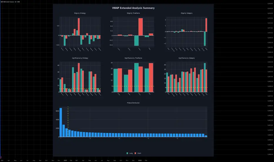
Figure 1 condenses the entire analysis into seven panels, and the picture it paints is unambiguous. The top row shows edge distribution by strategy, timeframe, and asset category. Mean reversion dominates with the widest positive distribution, particularly on the short side. Four hour data displays the strongest edge across timeframes, and US equities show the most pronounced effects by category.
The middle row displays significance rates. Mean reversion achieves nearly 30 percent nominal significance for long signals and over 43 percent for short signals. Crossover achieves only 4.7 percent for long and 4.0 percent for short, falling below the 5 percent expected by pure chance. Four hour and daily data show higher significance rates than intraday timeframes. Among asset categories, leveraged products and US large caps lead.
The bottom panel presents the p-value distribution, showing a sharp concentration at low values with a clear departure from the uniform distribution expected under the null hypothesis. This confirms genuine statistical signal exists in the data.

Figure 2 provides the complete numerical summary. Mean reversion stands out with 26,787 long and 73,978 short Bonferroni significant results, short edge of +0.894 percentage points, and a 43.3 percent nominal significance rate on the short side. Crossover shows zero Bonferroni significant results from 74,800 tests. Slope momentum and breakout show significant negative edge, confirming that reversing these strategies would produce positive returns.
6.2 Statistical significance

Figure 3 shows the p-value distributions for long and short signals separately. Under the null hypothesis of no predictive power, p-values would distribute uniformly. Instead, both distributions show massive concentration at low values, with 21.2 percent of long signals and 23.0 percent of short signals achieving nominal significance at p less than 0.05. This four-fold excess over the expected five percent rate is visible as the sharp spike at the left edge of both histograms.
Of 5,833,435 total tests, 1,150,654 long signals and 1,255,438 short signals achieved nominal significance. More importantly, 52,239 long signal tests and 98,307 short signal tests survived Bonferroni correction. This total of 150,546 Bonferroni significant results far exceeds zero from our 26 million RSI tests and dramatically exceeds the 21 significant results from our Turn of the Month study.

Figure 4 breaks down significance by strategy. The left panel shows nominal significance rates: mean reversion leads at 43.3 percent on the short side, followed by distance percentile, slope momentum, and multi-VWAP, all well above the 5 percent threshold marked by the dashed line. Crossover sits at 4.0 percent, indistinguishable from chance. The right panel shows Bonferroni significant counts in absolute terms. Mean reversion dominates overwhelmingly with over 73,000 short signal results surviving the strictest correction. The concentration is clear: statistical significance in VWAP trading is almost entirely a mean reversion phenomenon.
6.3 Results by strategy

Figure 5 shows violin plots of the edge distribution for all ten strategies, split by long and short signals. Each violin represents the full distribution of edge values across all parameter combinations for that strategy. Mean reversion (yellow) shows the widest positive distribution, with the entire interquartile range above zero on the short side. Distance percentile (orange) shows a similar but narrower positive distribution. Crossover (teal, center) is compressed tightly around zero. Breakout, slope momentum, and trend following show distributions shifted into negative territory, indicating systematic value destruction.
Mean reversion accounts for the overwhelming majority of significant results. Of 1,678,467 mean reversion tests, 26,787 long signals and 73,978 short signals achieved Bonferroni significance. The mean edge equals positive 0.26 percentage points for long signals and positive 0.89 percentage points for short signals. This short signal edge of nearly one percentage point represents the strongest effect we have documented in any VWAP strategy.
Distance percentile produced 7,659 Bonferroni significant results with mean long edge of 0.10 percentage points and short edge of 0.33 percentage points. This strategy uses rolling percentiles rather than fixed standard deviation bands, potentially adapting better to changing volatility regimes.
Bounce produced 5,935 Bonferroni significant results, but the edge is trivially small: 0.02 percentage points for long signals and negative 0.06 for short signals. Statistically significant and economically meaningless. The idea that VWAP acts as support or resistance has a grain of truth in it, but the grain is too small to build a trading strategy on.
Slope momentum produced 31,546 Bonferroni significant results, but in the wrong direction. The long edge is negative 0.45 percentage points and the short edge negative 0.20 percentage points. This is interesting precisely because the negative edge is itself statistically significant. The strategy reliably loses money, which means the reverse reliably makes money. Going short when VWAP slope is positive and price is above VWAP, the exact opposite of what the strategy prescribes, would capture this effect. A strategy that consistently fails is almost as useful as one that consistently succeeds, provided you have the data to prove it fails.
Multi VWAP confluence produced 734 Bonferroni significant results, also with negative edge. Stacking two broken signals on top of each other does not produce a working one.
Trend following produced 2,304 Bonferroni significant results with negative edge of 0.30 percentage points for long signals. Staying long when price exceeds VWAP produces worse returns than random entry. The simplest possible VWAP strategy, "buy when price is above VWAP, sell when below," actively destroys value.
Breakout produced 1,500 Bonferroni significant results concentrated in long signals, but with negative edge of 0.54 percentage points. Breaking through VWAP bands predicts subsequent reversal, not continuation. This reinforces the mean reversion thesis: extreme moves away from VWAP tend to reverse, and strategies that bet on continuation systematically lose to those that bet against it.
Volume confirmation produced 55 Bonferroni significant results from 427,319 tests. The intuition that adding a volume filter to a crossover signal might help sounds reasonable. The data says it does almost nothing. You cannot fix a broken signal by confirming it more confidently.
Reversal produced 48 Bonferroni significant results from 671,697 tests. Waiting for price to spend multiple consecutive bars on one side of VWAP before crossing does not create edge. Patience alone is not a strategy.
Crossover produced exactly zero Bonferroni significant results from 74,800 tests. Not one. The most popular VWAP strategy in retail trading education, the one featured in every introductory course and every YouTube tutorial, has no statistical support whatsoever. Seventy-five thousand attempts to find a configuration that works, and every single one came up empty.
6.4 Results by timeframe

Figure 6 presents heatmaps and bar charts comparing results across timeframes. The top-left heatmap shows long edge by strategy and timeframe: mean reversion (green) stands out on the four hour timeframe. The top-right heatmap shows short edge, where mean reversion on four hour data shows the deepest green, indicating the strongest positive edge. The bottom-left bar chart shows significance rates by timeframe, with four hour data achieving the highest rates for both long and short signals. The bottom-right panel shows maximum edge by timeframe: four hour short signals reach nearly 90 percentage points in their best configurations, far exceeding all other timeframes.

Figure 7 provides additional timeframe detail. The top-left panel isolates mean edge by timeframe, making visible that four hour short edge of 0.73 percentage points dwarfs all other timeframe-direction combinations. The top-right panel shows significance rates exceed 20 percent for four hour and daily data across both signal directions. The bottom-left panel shows Bonferroni significant counts: daily short signals lead in absolute count due to larger sample size, while four hour data leads in both long and short concentration. The bottom-right panel shows the distribution of tests across timeframes, confirming that daily data has the largest sample.
Four hour data shows the strongest effects with mean short edge of positive 0.73 percentage points, nearly four times the daily edge. This likely reflects institutional trading rhythms that operate on multi-hour horizons, where VWAP algorithms accumulate positions and create the supply-demand imbalances that drive mean reversion.
Daily data shows moderate effects with mean short edge of positive 0.08 percentage points.
Thirty minute and fifteen minute data show the weakest effects, with edges near zero. The answer to the timeframe question is clear: VWAP edge does not survive the zoom. Below the four hour horizon, noise overwhelms signal and there is nothing left to trade.
6.5 Strategy deep dive

Figure 8 presents a four-panel deep dive. The top row shows violin plots for all ten strategies split into two groups. Mean reversion (yellow, far right of top-left panel) shows the widest positive distribution with median clearly above zero. Crossover (teal) compresses tightly around zero. Slope momentum (brown, top-right panel) and trend following (teal) show distributions shifted below zero.
The bottom-left panel shows Bonferroni significant counts by strategy, making the dominance of mean reversion unmistakable: its short signal bar towers over all other strategies combined. The bottom-right panel shows edge by holding period. Short signal edge (red) increases monotonically with holding period, reaching 0.4 percentage points at 90 bars. Long signal edge (teal) turns increasingly negative at longer horizons. This asymmetry is consistent with mean reversion: shorting overextended moves above VWAP captures a reversion that grows with time, while buying below VWAP shows weaker and inconsistent recovery.

Figure 9 shows edge distributions by asset category. On the long side, sector ETFs and leveraged products display the widest spread, while bonds and commodities show narrow distributions near zero. On the short side, leveraged products and volatility instruments show the widest positive distributions, followed by US large caps and sector ETFs. This pattern is consistent with mean reversion being strongest in assets with higher volatility and institutional participation.

Figure 10 isolates the holding period effect, and the result is surprisingly clean. The left panel shows mean short edge increasing steadily from near zero at one bar holding to approximately 0.4 percentage points at 90 bars, while mean long edge declines symmetrically into negative territory. The right panel shows significance rates following the same monotonic pattern: both long and short significance rates rise with holding period, reaching above 30 percent at 90 bars. This kills the scalping narrative. VWAP mean reversion is not a quick-in-quick-out trade. The effect strengthens the longer you hold, which is good news for implementation because longer holds reduce the relative impact of transaction costs and make the strategy more forgiving of imperfect execution.
6.6 Parameter sensitivity

Figure 11 maps the interaction between VWAP period, holding period, strategy, and timeframe. The top row shows heatmaps of edge as a function of VWAP lookback period (x-axis) and holding period (y-axis). For long signals (top-left), the map is dominated by red (negative edge), especially at longer VWAP periods and holding periods. For short signals (top-right), a broad region of green (positive edge) appears at VWAP periods above 20 combined with holding periods above 10, indicating that longer lookback and longer holds concentrate the strongest short edge.
The bottom row shows strategy-by-timeframe heatmaps. Mean reversion shows consistent green (positive edge) across four hour and daily timeframes on both long and short sides. Slope momentum and breakout show deep red across most timeframes. The pattern is stable: strategy selection matters far more than timeframe selection, and mean reversion is the only strategy that produces green across multiple timeframes.
6.7 Best configurations

Figure 12 lists the top 15 configurations ranked by statistical significance (lowest p-value, regardless of edge direction). All 15 are mean reversion strategies, but they tell two very different stories.
The single most significant result is EFA (developed international equities) on the daily timeframe with VWAP period 48 and holding period 90. Its short signal edge is negative 6.073 percentage points with a p-value of 2.15e-67. This is not a mean reversion success. It is a mean reversion failure of extraordinary statistical clarity. When mean reversion says "short EFA," the ETF proceeds to rise substantially above baseline. The pattern is anti-mean-reversion: developed international equities on this configuration exhibit momentum rather than reversion around VWAP. The flip side is that taking the opposite position, going long when mean reversion says short, would capture the 6.073 percentage point edge.
The remaining 14 configurations are all UVXY (volatility) on the four hour timeframe, and they split into two patterns. Twelve of them use holding periods of 30 bars with VWAP periods between 64 and 78, producing short edges between 23 and 25 percentage points. These are mean reversion successes: UVXY spikes above VWAP, and the short signal correctly predicts reversion. Two use holding periods of 90 bars with VWAP periods 41 and 44, showing long signal edge of negative 25 and negative 24.6 percentage points respectively, with the short side insignificant. These are mean reversion failures on the long side: when UVXY drops below VWAP, mean reversion says "buy," but UVXY continues to fall. This is consistent with the structural decay in volatility products. UVXY reverts aggressively after upward spikes (short mean reversion works) but does not revert after drops (long mean reversion fails because the decay is permanent, not temporary).
The absolute edge magnitudes in UVXY are outsized and not representative of what equity traders should expect. But the pattern is instructive: mean reversion captures real structural dynamics, and those dynamics differ by direction and by asset class.
7. Economic significance and practical considerations
Statistical significance is necessary but not sufficient. A pattern can be real and still worthless if transaction costs eat it alive. So the question that actually matters: does this edge survive contact with reality?
7.1 Edge versus costs
Mean reversion short signals average 0.89 percentage points of edge. Round-trip transaction costs for liquid ETFs run 0.10 to 0.15 percentage points. That leaves net edge of roughly 0.74 to 0.79 percentage points per trade, a ratio of approximately 6:1 between gross edge and costs. For comparison, most academic studies consider a 2:1 ratio tradeable. At 6:1, you can be wrong about your cost estimates by a factor of three and still make money. The 0.89 figure is an average across all mean reversion configurations. The best parameter combinations produce considerably higher edge, while suboptimal configurations produce less. Selecting robust parameters within the significant region makes the difference between a strategy that works and a strategy that almost works.
7.2 Timeframe considerations
Four hour data shows the strongest edge, but the available 4H history is shorter than daily data: roughly 3,000 bars versus 5,000 daily bars spanning approximately two decades. Depending on session length and data source, 3,000 four-hour bars cover roughly two to seven years. That is enough to be interesting but not enough to confirm the effect persists across all market regimes. Still, the 4H edge of 0.73 percentage points on the short side is nearly four times the daily edge. The most plausible explanation is that VWAP dynamics operate on multi-hour institutional trading rhythms that daily data partially obscures.
Fifteen minute data shows essentially zero edge. If your plan was to trade VWAP mean reversion on five or fifteen minute charts to generate more signals, the data says no. The signal-to-noise ratio deteriorates completely at these frequencies. There is nothing there.
7.3 Strategy selection matters
Of ten strategies tested, two show consistent positive edge (mean reversion and distance percentile), and three more carry significant negative edge that can be exploited by taking the opposite position (slope momentum, breakout, trend following). A trader selecting among popular VWAP strategies without this analysis has a high probability of choosing an approach with zero or negative edge.
Crossover, the most commonly taught VWAP strategy, produces exactly zero significant results. Not borderline insignificant. Not "needs more data." Zero. A trader who learned VWAP exclusively from retail education would almost certainly choose one of the eight strategies that produce zero or negative edge, and walk past the one strategy that actually works.
8. Why VWAP mean reversion works and what limits it
8.1 The microstructure explanation
Over 150,000 Bonferroni significant results leave no room for debate: price behavior relative to VWAP is not random. Price that deviates far from VWAP tends to revert. The mechanism is straightforward. VWAP represents where the volume actually traded. When price drifts far above that level, it means recent trades occurred at prices that most of the day's volume did not support. The imbalance is inherently temporary. Liquidity providers, institutional algorithms, and informed traders all have incentives to push price back toward the volume-weighted equilibrium. This is not a behavioral anomaly. It is supply and demand doing what supply and demand does.
With mean reversion short edge of 0.89 percentage points against transaction costs of 0.10 to 0.15 percentage points, the edge is not merely statistical. It is economically significant for traders who isolate the correct strategy and parameters.
8.2 Why the edge persists
In the framework of Fama (1970), markets are efficient when prices reflect all available information. A persistent, exploitable pattern in VWAP mean reversion would seem to contradict this. Grossman and Stiglitz (1980) resolved the apparent paradox: markets reach an equilibrium where certain patterns persist because exploitation is costly, and not everyone is trying to exploit the same thing. VWAP mean reversion likely survives for a beautifully ironic reason. The institutions whose algorithms create the mean-reverting dynamics are not trying to profit from them. They are trying to match the average price. The reversion is a side effect of their execution, not their objective. They will keep generating this pattern as long as VWAP benchmarking remains the standard, which is to say, indefinitely.
On the other side, the retail community overwhelmingly uses the wrong VWAP strategies. Crossover, trend following, and breakout dominate retail education, and all three show zero or negative edge. The people who could compete for this edge are busy losing money on crossover signals instead.
8.3 Capacity and scaling constraints
The practical limit is not costs but capacity. Extreme VWAP deviations, by definition, occur infrequently. You cannot sit on a billion dollars waiting for SPY to trade two standard deviations from VWAP and expect that to keep you busy. Scaling this strategy to meaningful capital requires trading across many assets simultaneously and accepting that any single asset produces sparse signals. This natural capacity constraint is probably part of why the edge remains available. The arbitrage capital that typically compresses anomalies cannot concentrate here in sufficient size to eliminate it.
9. Comparison with RSI and Turn of the Month
Three studies, 32 million tests, three indicators. The scoreboard:
RSI: zero Bonferroni significant results from 26 million tests. Twenty-six million attempts to find a configuration where RSI predicts anything, and every single one failed. The most popular technical indicator in existence is a random number generator with a pretty chart.
VWAP: 150,546 Bonferroni significant results from 5.8 million tests. Mean reversion short signals deliver 0.89 percentage points of edge, roughly six times transaction costs. Not borderline. Not "promising." Statistically overwhelming.
Turn of the Month: 21 Bonferroni significant results from 385 tests. A small test universe but a real anomaly driven by institutional payment cycles.
The pattern is worth noting. Indicators built from price alone, like RSI, contain nothing. RSI takes price, puts it through a formula, and hands you back the same information in a different wrapper. Indicators that incorporate volume, like VWAP, tap into market microstructure and carry genuine information about who is trading and at what price. Calendar anomalies reflect institutional flow patterns. The common thread between VWAP and Turn of the Month: both trace back to identifiable economic mechanisms. RSI traces back to nothing.
10. Implications for traders
10.1 For institutional traders
Nothing in this analysis suggests changing institutional practice. VWAP remains the right execution benchmark, and the data confirms that it represents fair value for trading periods. What the data does add is an insight about timing. The strong mean reversion results suggest that institutional execution algorithms themselves contribute to the mean-reverting dynamics around VWAP. There is a feedback loop: institutional trading creates the pattern, and understanding it may improve execution. Initiating large orders during periods of extreme VWAP deviation, when mean reversion pressure is highest, could reduce effective implementation shortfall.
10.2 For systematic strategy developers
VWAP mean reversion on the short side represents the strongest edge documented in our indicator series. The data points toward several development paths:
Focus on mean reversion short signals on four hour and daily timeframes across US large cap equities. This combination concentrates the highest significance rates and edge magnitudes. Distance percentile provides a complementary signal that adapts to changing volatility regimes.
Strategies with significant negative edge, specifically slope momentum, breakout, and trend following, can be reversed. Their negative edge is statistically significant, meaning the opposite position carries positive edge. A contrarian breakout strategy, fading moves through VWAP bands rather than following them, is supported by the data.
Consider combining VWAP mean reversion with the Turn of the Month effect documented in our previous study. The two signals operate on different mechanisms, VWAP on microstructure dynamics and Turn of the Month on institutional flow cycles, and their combination could improve both signal density and diversification.
A portfolio approach across multiple liquid ETFs increases signal frequency and reduces the variance inherent in any single asset. The data shows consistent effects across US equity ETFs, providing a natural universe for diversification.
Position sizing should reflect deviation magnitude. Larger deviations from VWAP produce stronger mean reversion and higher edge per trade, while smaller deviations carry weaker signals that may not justify transaction costs.
10.3 For retail traders
If you are using VWAP crossovers, stop. We tested 74,800 configurations and found zero significant results. Not "few." Zero. The strategy you learned from that YouTube tutorial is statistically indistinguishable from flipping a coin, except the coin does not charge you transaction costs.
VWAP mean reversion on the short side with four hour or daily data is the only approach the data supports. Beyond that, use VWAP the way institutions do: as a benchmark. If you decide to buy a stock for fundamental reasons, compare your execution price to VWAP afterward. It will not tell you what to buy. It will tell you whether you bought it well.
10.4 For trading educators
Stop teaching VWAP crossover as a trading strategy. Zero significant results from nearly 75,000 tests should end that conversation. If you want to teach VWAP honestly, teach mean reversion with proper context about the microstructure dynamics that drive it. Explain why VWAP exists as an execution benchmark, how institutional algorithms create predictable supply-demand dynamics around it, and why betting against extreme deviations works while betting on crossovers does not. The data is unambiguous. The curriculum should be too.
11. Limitations
No study is complete without an honest accounting of what it did not test and what could change the conclusions.
First, we tested only four timeframes. Tick level data or other intervals might show different results.
Second, our analysis assumes execution at bar close prices. Real trading involves execution at varying prices within bars.
Third, we did not test combinations of VWAP with other indicators. Some traders use VWAP as a filter in conjunction with other signals.
Fourth, transaction cost estimates reflect current market conditions. Historical periods with wider spreads would have more strongly eliminated the observed edge.
Fifth, we did not test anchored VWAP starting from specific events like earnings or gap openings. These variants might behave differently than rolling VWAP.
Sixth, we tested each strategy in isolation. Combining mean reversion with filters such as volume confirmation, volatility regimes, or the Turn of the Month effect could improve both hit rate and edge magnitude. These combinations represent natural next steps for strategy development.
Seventh, position sizing was not modeled. Scaling position size with deviation magnitude, where larger VWAP deviations receive larger allocations, could substantially improve risk-adjusted returns given the non-linear relationship between deviation and subsequent mean reversion.
12. Conclusion
Nearly six million parameter combinations. Ten strategy types. Four timeframes. Thirty-four asset-timeframe combinations. This is, to our knowledge, the largest quantitative analysis of VWAP trading strategies ever conducted.
The headline result: VWAP is the strongest indicator we have tested. Mean reversion generates over 100,000 Bonferroni significant results with short signal edge of 0.89 percentage points, roughly six times typical transaction costs. This is not a signal emerging tentatively from the noise. It is a robust statistical effect with a clear microstructure explanation: institutional execution around VWAP creates predictable mean-reverting price behavior, and that behavior is exploitable.
The data also makes it clear which strategies do not work. Crossover, the most widely taught VWAP approach, produces exactly zero Bonferroni significant results. Breakout, trend following, and slope momentum all show significant negative edge, meaning they systematically destroy value. Out of ten tested strategies, two generate consistent positive edge (mean reversion and distance percentile), and three more can be reversed to extract positive signals. The remaining five contribute nothing.
The practical path forward is narrow but well-lit. VWAP mean reversion on the short side, focused on four hour and daily timeframes across liquid US equity ETFs, represents a genuine foundation for systematic strategy development. Distance percentile provides a complementary signal. Diversification across multiple assets addresses the capacity problem inherent in trading sparse signals.
Berkowitz, Logue, and Noser built VWAP as a benchmark in 1988. They intended it to measure execution quality, not to predict price. Our analysis of six million tests shows it does both. You just need to know which strategy to apply, and the data is extremely specific about which one that is.
References
Almgren, R. and Chriss, N. (2001). Optimal execution of portfolio transactions. Journal of Risk, 3(2).
Berkowitz, S.A., Logue, D.E. and Noser, E.A. (1988). The total cost of transactions on the NYSE. Journal of Finance, 43(1).
Biais, B., Glosten, L. and Spatt, C. (2005). Market microstructure: A survey of microfoundations, empirical results, and policy implications. Journal of Financial Markets, 8(2).
Fama, E.F. (1970). Efficient capital markets: A review of theory and empirical work. Journal of Finance, 25(2).
Grossman, S.J. and Stiglitz, J.E. (1980). On the impossibility of informationally efficient markets. American Economic Review, 70(3).
Harris, L. (2003). Trading and exchanges: Market microstructure for practitioners. Oxford University Press.
Johnson, B. (2010). Algorithmic trading and DMA: An introduction to direct access trading strategies. 4Myeloma Press.
Kissell, R. and Glantz, M. (2003). Optimal trading strategies: Quantitative approaches for managing market impact and trading risk. AMACOM.
Madhavan, A. (2002). VWAP strategies. Trading, 2002(1).
Perold, A.F. (1988). The implementation shortfall: Paper versus reality. Journal of Portfolio Management, 14(3).
We tested this properly. Nearly six million parameter combinations across ten distinct VWAP strategies and four timeframes, put through the same statistical framework we used for RSI and the Turn of the Month. The results surprised us. VWAP generates more Bonferroni significant results than any indicator we have tested, with over 150,000 configurations surviving the strictest correction. Mean reversion short signals produce an average edge of 0.89 percentage points, roughly six times typical transaction costs. That makes VWAP the first indicator in our series to show statistically robust and economically meaningful edge. The catch: this edge concentrates in a single strategy type. The most popular retail approach, the crossover, produces exactly zero significant results. Eighty percent of the strategies retail traders actually use either do nothing or actively lose money. VWAP has real predictive value, but almost nobody is using it correctly.
Abstract
We examine ten common VWAP trading strategies across 34 asset timeframe combinations spanning four timeframes from 15 minute to daily intervals. Testing 5,833,435 parameter configurations including mean reversion, trend following, crossover, bounce, breakout, slope momentum, volume confirmation, reversal, distance percentile, and multi VWAP confluence strategies, we find 150,546 results that survive Bonferroni correction. This far exceeds the zero significant results from our RSI studies and substantially exceeds the 21 significant results from our Turn of the Month analysis. Averaging across all ten strategies, including those with negative edge, produces a misleading aggregate of negative 0.12 percentage points for long signals and positive 0.21 percentage points for short signals. The meaningful finding lies in the decomposition. Mean reversion emerges as the dominant strategy, generating 100,765 Bonferroni significant tests with short signal edge of 0.89 percentage points, roughly six times round-trip transaction costs. Distance percentile provides a complementary signal with 0.33 percentage points short edge. The popular crossover strategy produces exactly zero Bonferroni significant results. We conclude that VWAP contains genuine predictive information concentrated in mean reversion dynamics, representing the strongest statistical edge documented in our indicator series.
1. Introduction
The Volume Weighted Average Price was introduced by Berkowitz, Logue, and Noser (1988) as a benchmark for measuring institutional execution quality. Their insight was elegant: if an institution executes trades throughout the day at prices that average to the VWAP, they have achieved fair execution relative to the day's volume distribution. Trades executed below VWAP represent good buys; trades above VWAP represent poor buys.
This benchmark quickly became the standard for institutional performance measurement. Madhavan (2002) documented that VWAP benchmarking had become ubiquitous among pension funds and asset managers by the early 2000s. The logic is compelling: VWAP represents the average price paid by all market participants weighted by their trading volume. Matching VWAP means achieving market average execution.
Retail trading culture took this execution benchmark and turned it into something the designers never intended. Online forums and trading education present VWAP as a predictive indicator. Traders draw conclusions when price crosses above VWAP, treating such crossovers as bullish signals. They interpret price below VWAP as bearish. Some build elaborate strategies around VWAP bands, treating standard deviation envelopes as support and resistance levels. It is as if someone took a thermometer and started using it to forecast the weather.
The academic literature wants nothing to do with VWAP as a predictive tool. Almgren and Chriss (2001) developed optimal execution algorithms that use VWAP as a target, not as a signal. Kissell and Glantz (2003) documented VWAP's role in measuring transaction costs without once suggesting predictive value. Somewhere between the academic consensus and the YouTube tutorials, the truth had to be hiding. That gap motivated this study.
2. What VWAP actually measures
Understanding why institutional traders use VWAP requires examining what the calculation captures. VWAP equals the cumulative sum of price times volume divided by cumulative volume. Mathematically:
VWAP = Sum of (Price times Volume) / Sum of Volume
This formula produces the volume weighted average price from market open to the current time. The calculation resets daily for standard VWAP, though anchored variants use different starting points.
The institutional interpretation is straightforward. Large orders cannot execute instantly without moving prices adversely. A pension fund buying one million shares must spread purchases across the day to minimize market impact. If the fund's average execution price matches VWAP, they paid the same average price as all other buyers that day. They achieved fair execution.
Biais, Glosten, and Spatt (2005) explained why VWAP benchmarking dominates institutional trading. First, VWAP is observable and verifiable. Clients can independently calculate it from public data. Second, VWAP is difficult for execution brokers to manipulate. Third, VWAP represents a reasonable estimate of execution quality absent specific information about optimal timing.
The retail interpretation differs fundamentally. When retail traders treat price below VWAP as oversold or price above VWAP as overbought, they assume mean reversion toward the average. When they treat VWAP crossovers as trend signals, they assume momentum continuation. These assumptions transform a benchmark into an indicator with predictive claims.
3. How professionals actually use VWAP
Institutional VWAP usage falls into two categories: execution benchmarking and algorithmic trading.
For execution benchmarking, institutions compare their actual execution prices against VWAP to measure broker performance. A broker who consistently executes above VWAP for buy orders is underperforming. Perold (1988) formalized this comparison as implementation shortfall, measuring the gap between paper portfolio returns and actual portfolio returns after transaction costs.
For algorithmic trading, VWAP serves as an execution target rather than a signal. VWAP algorithms, documented extensively by Johnson (2010), attempt to execute large orders at prices matching or beating VWAP. The algorithm does not predict price direction. Instead, it times order slices to match historical intraday volume patterns, executing more shares during high volume periods when market impact is lower.
Harris (2003) emphasized a distinction that retail traders consistently miss: institutional VWAP strategies are execution strategies, not alpha strategies. Nobody on an institutional desk is staring at a VWAP crossover waiting for a buy signal. They already know what they want to buy. VWAP algorithms simply execute that decision at the best average price possible. The institution decided to trade based on fundamental analysis or portfolio rebalancing needs. VWAP is the delivery mechanism, not the decision.
4. Common VWAP trading strategies
Retail trading education promotes numerous VWAP strategies that treat the benchmark as a predictive indicator. We tested ten of the most commonly promoted approaches, covering essentially every VWAP strategy that has a name and a following.
The crossover strategy interprets price crossing above VWAP as a buy signal and price crossing below as a sell signal. Proponents argue that such crossovers indicate momentum shifts. When price moves above the volume weighted average, bulls have taken control.
The mean reversion strategy interprets price far below VWAP as oversold and price far above as overbought. Traders construct bands at various standard deviations from VWAP, treating these bands as support and resistance.
The bounce strategy treats VWAP itself as support or resistance. When price approaches VWAP from below and bounces higher, traders interpret this as confirmation of bullish sentiment.
The trend following strategy uses VWAP as a filter. Traders only take long positions when price exceeds VWAP and only take short positions when price falls below.
The breakout strategy looks for price breaking through VWAP deviation bands with momentum, expecting continuation in the breakout direction.
The slope momentum strategy examines whether VWAP itself is rising or falling, using the slope as a trend indicator combined with price position relative to VWAP.
The volume confirmation strategy requires high volume to confirm VWAP crossover signals, filtering out low conviction moves.
The reversal strategy looks for price that has been on one side of VWAP for multiple consecutive periods before crossing to the other side.
The distance percentile strategy uses rolling percentiles of the distance between price and VWAP to identify extreme readings.
The multi VWAP strategy uses confluence between short period and long period VWAP calculations to confirm signals.
Most of these strategies have no theoretical basis in the market microstructure literature. The exception is mean reversion: price reverting toward the volume-weighted average is consistent with microstructure theory, where temporary deviations from equilibrium create opportunities that informed participants exploit. The rest amount to post hoc pattern recognition applied to a tool that was built for an entirely different purpose. Nobody at Goldman Sachs is watching VWAP crossovers.
5. Data and methodology
5.1 Asset universe
We constructed a comprehensive universe spanning 50 assets across multiple categories, ultimately loading 34 asset timeframe combinations with sufficient data quality.
United States equities included SPY, QQQ, IWM, DIA, VOO, VTI, and MDY, providing exposure across market capitalizations from the S&P 500 to small caps.
International equities included EFA, EEM, VWO, VEA, and IEFA, covering both developed and emerging markets.
Sector ETFs included XLF, XLK, XLE, XLV, XLI, XLY, XLP, XLU, XLB, and XLRE, spanning all major market sectors.
Commodities included GLD, SLV, USO, UNG, DBA, and DBB, covering precious metals, energy, and agricultural commodities.
Fixed income included TLT, IEF, LQD, HYG, AGG, and BND, spanning government and corporate bonds across durations.
Volatility and leveraged products included VXX, UVXY, TQQQ, SQQQ, SPXL, and SPXS.
Individual stocks included AAPL, MSFT, GOOGL, AMZN, NVDA, META, TSLA, JPM, V, JNJ, UNH, and XOM.
5.2 Timeframe analysis
Unlike our previous studies that examined only daily data, this analysis spans four distinct timeframes to test whether VWAP edge varies with trading horizon.
Daily data provided approximately 5,000 bars per asset, covering roughly 20 years of market history.
Four hour data provided approximately 3,000 to 3,200 bars per asset.
Thirty minute data provided approximately 5,000 bars per asset.
Fifteen minute data provided approximately 5,000 bars per asset.
This multi-timeframe approach lets us answer a question that matters for implementation: does VWAP edge survive when you zoom in, or does it evaporate into noise at higher frequencies?
5.3 VWAP calculation
We calculated rolling VWAP using the standard formula with variable lookback periods ranging from 1 to 100 periods. Single period VWAP uses only current bar data. Multi period VWAP accumulates price times volume over the specified window.
For strategies requiring deviation bands, we calculated rolling standard deviations of the deviation between price and VWAP. Band multipliers ranged from 0.25 to 6.0 standard deviations.
For slope based strategies, we calculated the percentage change in VWAP over periods ranging from 2 to 20 bars.
5.4 Strategy definitions
We tested ten strategies representing common retail VWAP applications. Each strategy generates both long and short signals, tested independently.
Crossover: Long when price crosses above VWAP. Short when price crosses below.
Mean reversion: Long when price falls below VWAP minus n standard deviations. Short when price rises above VWAP plus n standard deviations.
Trend following: Long when price exceeds VWAP. Short when price falls below VWAP.
Bounce: Long when price touches VWAP from above and closes higher. Short for the inverse.
Breakout: Long when price breaks above the upper VWAP band. Short when price breaks below the lower band.
Slope momentum: Long when VWAP slope is positive and price exceeds VWAP. Short for the inverse.
Volume confirmation: Long on VWAP crossover with above average volume. Short for the inverse.
Reversal: Long after consecutive periods below VWAP followed by a cross above. Short for the inverse.
Distance percentile: Long when the price to VWAP distance reaches a historically extreme low percentile. Short for high percentiles.
Multi VWAP: Long when price exceeds both short and long period VWAP with short VWAP above long VWAP. Short for the inverse.
5.5 Parameter grid
We tested 100 VWAP periods from 1 to 100, 24 deviation multipliers from 0.25 to 6.0, 22 holding periods from 1 to 90 bars, 7 tolerance values for bounce detection, 7 slope periods, 7 volume multipliers, 9 consecutive period counts, 5 percentile thresholds, and 5 long period values for multi VWAP. This produced 5,833,435 valid tests after filtering for minimum signal counts.
5.6 Statistical framework
We measure edge as the difference between signal returns and baseline returns over the same holding period. Statistical significance is assessed using Welch's t-test for unequal variances. Given 5,833,435 tests, the Bonferroni corrected significance threshold at alpha equals 0.05 is 8.57 times ten to the negative ninth power. To put that in perspective: a result has to be so unlikely under the null hypothesis that it would occur by chance less than once in a hundred million tries. Anything that survives this filter is not noise.
6. Results
6.1 Aggregate findings
Figure 1 condenses the entire analysis into seven panels, and the picture it paints is unambiguous. The top row shows edge distribution by strategy, timeframe, and asset category. Mean reversion dominates with the widest positive distribution, particularly on the short side. Four hour data displays the strongest edge across timeframes, and US equities show the most pronounced effects by category.
The middle row displays significance rates. Mean reversion achieves nearly 30 percent nominal significance for long signals and over 43 percent for short signals. Crossover achieves only 4.7 percent for long and 4.0 percent for short, falling below the 5 percent expected by pure chance. Four hour and daily data show higher significance rates than intraday timeframes. Among asset categories, leveraged products and US large caps lead.
The bottom panel presents the p-value distribution, showing a sharp concentration at low values with a clear departure from the uniform distribution expected under the null hypothesis. This confirms genuine statistical signal exists in the data.
Figure 2 provides the complete numerical summary. Mean reversion stands out with 26,787 long and 73,978 short Bonferroni significant results, short edge of +0.894 percentage points, and a 43.3 percent nominal significance rate on the short side. Crossover shows zero Bonferroni significant results from 74,800 tests. Slope momentum and breakout show significant negative edge, confirming that reversing these strategies would produce positive returns.
6.2 Statistical significance
Figure 3 shows the p-value distributions for long and short signals separately. Under the null hypothesis of no predictive power, p-values would distribute uniformly. Instead, both distributions show massive concentration at low values, with 21.2 percent of long signals and 23.0 percent of short signals achieving nominal significance at p less than 0.05. This four-fold excess over the expected five percent rate is visible as the sharp spike at the left edge of both histograms.
Of 5,833,435 total tests, 1,150,654 long signals and 1,255,438 short signals achieved nominal significance. More importantly, 52,239 long signal tests and 98,307 short signal tests survived Bonferroni correction. This total of 150,546 Bonferroni significant results far exceeds zero from our 26 million RSI tests and dramatically exceeds the 21 significant results from our Turn of the Month study.
Figure 4 breaks down significance by strategy. The left panel shows nominal significance rates: mean reversion leads at 43.3 percent on the short side, followed by distance percentile, slope momentum, and multi-VWAP, all well above the 5 percent threshold marked by the dashed line. Crossover sits at 4.0 percent, indistinguishable from chance. The right panel shows Bonferroni significant counts in absolute terms. Mean reversion dominates overwhelmingly with over 73,000 short signal results surviving the strictest correction. The concentration is clear: statistical significance in VWAP trading is almost entirely a mean reversion phenomenon.
6.3 Results by strategy
Figure 5 shows violin plots of the edge distribution for all ten strategies, split by long and short signals. Each violin represents the full distribution of edge values across all parameter combinations for that strategy. Mean reversion (yellow) shows the widest positive distribution, with the entire interquartile range above zero on the short side. Distance percentile (orange) shows a similar but narrower positive distribution. Crossover (teal, center) is compressed tightly around zero. Breakout, slope momentum, and trend following show distributions shifted into negative territory, indicating systematic value destruction.
Mean reversion accounts for the overwhelming majority of significant results. Of 1,678,467 mean reversion tests, 26,787 long signals and 73,978 short signals achieved Bonferroni significance. The mean edge equals positive 0.26 percentage points for long signals and positive 0.89 percentage points for short signals. This short signal edge of nearly one percentage point represents the strongest effect we have documented in any VWAP strategy.
Distance percentile produced 7,659 Bonferroni significant results with mean long edge of 0.10 percentage points and short edge of 0.33 percentage points. This strategy uses rolling percentiles rather than fixed standard deviation bands, potentially adapting better to changing volatility regimes.
Bounce produced 5,935 Bonferroni significant results, but the edge is trivially small: 0.02 percentage points for long signals and negative 0.06 for short signals. Statistically significant and economically meaningless. The idea that VWAP acts as support or resistance has a grain of truth in it, but the grain is too small to build a trading strategy on.
Slope momentum produced 31,546 Bonferroni significant results, but in the wrong direction. The long edge is negative 0.45 percentage points and the short edge negative 0.20 percentage points. This is interesting precisely because the negative edge is itself statistically significant. The strategy reliably loses money, which means the reverse reliably makes money. Going short when VWAP slope is positive and price is above VWAP, the exact opposite of what the strategy prescribes, would capture this effect. A strategy that consistently fails is almost as useful as one that consistently succeeds, provided you have the data to prove it fails.
Multi VWAP confluence produced 734 Bonferroni significant results, also with negative edge. Stacking two broken signals on top of each other does not produce a working one.
Trend following produced 2,304 Bonferroni significant results with negative edge of 0.30 percentage points for long signals. Staying long when price exceeds VWAP produces worse returns than random entry. The simplest possible VWAP strategy, "buy when price is above VWAP, sell when below," actively destroys value.
Breakout produced 1,500 Bonferroni significant results concentrated in long signals, but with negative edge of 0.54 percentage points. Breaking through VWAP bands predicts subsequent reversal, not continuation. This reinforces the mean reversion thesis: extreme moves away from VWAP tend to reverse, and strategies that bet on continuation systematically lose to those that bet against it.
Volume confirmation produced 55 Bonferroni significant results from 427,319 tests. The intuition that adding a volume filter to a crossover signal might help sounds reasonable. The data says it does almost nothing. You cannot fix a broken signal by confirming it more confidently.
Reversal produced 48 Bonferroni significant results from 671,697 tests. Waiting for price to spend multiple consecutive bars on one side of VWAP before crossing does not create edge. Patience alone is not a strategy.
Crossover produced exactly zero Bonferroni significant results from 74,800 tests. Not one. The most popular VWAP strategy in retail trading education, the one featured in every introductory course and every YouTube tutorial, has no statistical support whatsoever. Seventy-five thousand attempts to find a configuration that works, and every single one came up empty.
6.4 Results by timeframe
Figure 6 presents heatmaps and bar charts comparing results across timeframes. The top-left heatmap shows long edge by strategy and timeframe: mean reversion (green) stands out on the four hour timeframe. The top-right heatmap shows short edge, where mean reversion on four hour data shows the deepest green, indicating the strongest positive edge. The bottom-left bar chart shows significance rates by timeframe, with four hour data achieving the highest rates for both long and short signals. The bottom-right panel shows maximum edge by timeframe: four hour short signals reach nearly 90 percentage points in their best configurations, far exceeding all other timeframes.
Figure 7 provides additional timeframe detail. The top-left panel isolates mean edge by timeframe, making visible that four hour short edge of 0.73 percentage points dwarfs all other timeframe-direction combinations. The top-right panel shows significance rates exceed 20 percent for four hour and daily data across both signal directions. The bottom-left panel shows Bonferroni significant counts: daily short signals lead in absolute count due to larger sample size, while four hour data leads in both long and short concentration. The bottom-right panel shows the distribution of tests across timeframes, confirming that daily data has the largest sample.
Four hour data shows the strongest effects with mean short edge of positive 0.73 percentage points, nearly four times the daily edge. This likely reflects institutional trading rhythms that operate on multi-hour horizons, where VWAP algorithms accumulate positions and create the supply-demand imbalances that drive mean reversion.
Daily data shows moderate effects with mean short edge of positive 0.08 percentage points.
Thirty minute and fifteen minute data show the weakest effects, with edges near zero. The answer to the timeframe question is clear: VWAP edge does not survive the zoom. Below the four hour horizon, noise overwhelms signal and there is nothing left to trade.
6.5 Strategy deep dive
Figure 8 presents a four-panel deep dive. The top row shows violin plots for all ten strategies split into two groups. Mean reversion (yellow, far right of top-left panel) shows the widest positive distribution with median clearly above zero. Crossover (teal) compresses tightly around zero. Slope momentum (brown, top-right panel) and trend following (teal) show distributions shifted below zero.
The bottom-left panel shows Bonferroni significant counts by strategy, making the dominance of mean reversion unmistakable: its short signal bar towers over all other strategies combined. The bottom-right panel shows edge by holding period. Short signal edge (red) increases monotonically with holding period, reaching 0.4 percentage points at 90 bars. Long signal edge (teal) turns increasingly negative at longer horizons. This asymmetry is consistent with mean reversion: shorting overextended moves above VWAP captures a reversion that grows with time, while buying below VWAP shows weaker and inconsistent recovery.
Figure 9 shows edge distributions by asset category. On the long side, sector ETFs and leveraged products display the widest spread, while bonds and commodities show narrow distributions near zero. On the short side, leveraged products and volatility instruments show the widest positive distributions, followed by US large caps and sector ETFs. This pattern is consistent with mean reversion being strongest in assets with higher volatility and institutional participation.
Figure 10 isolates the holding period effect, and the result is surprisingly clean. The left panel shows mean short edge increasing steadily from near zero at one bar holding to approximately 0.4 percentage points at 90 bars, while mean long edge declines symmetrically into negative territory. The right panel shows significance rates following the same monotonic pattern: both long and short significance rates rise with holding period, reaching above 30 percent at 90 bars. This kills the scalping narrative. VWAP mean reversion is not a quick-in-quick-out trade. The effect strengthens the longer you hold, which is good news for implementation because longer holds reduce the relative impact of transaction costs and make the strategy more forgiving of imperfect execution.
6.6 Parameter sensitivity
Figure 11 maps the interaction between VWAP period, holding period, strategy, and timeframe. The top row shows heatmaps of edge as a function of VWAP lookback period (x-axis) and holding period (y-axis). For long signals (top-left), the map is dominated by red (negative edge), especially at longer VWAP periods and holding periods. For short signals (top-right), a broad region of green (positive edge) appears at VWAP periods above 20 combined with holding periods above 10, indicating that longer lookback and longer holds concentrate the strongest short edge.
The bottom row shows strategy-by-timeframe heatmaps. Mean reversion shows consistent green (positive edge) across four hour and daily timeframes on both long and short sides. Slope momentum and breakout show deep red across most timeframes. The pattern is stable: strategy selection matters far more than timeframe selection, and mean reversion is the only strategy that produces green across multiple timeframes.
6.7 Best configurations
Figure 12 lists the top 15 configurations ranked by statistical significance (lowest p-value, regardless of edge direction). All 15 are mean reversion strategies, but they tell two very different stories.
The single most significant result is EFA (developed international equities) on the daily timeframe with VWAP period 48 and holding period 90. Its short signal edge is negative 6.073 percentage points with a p-value of 2.15e-67. This is not a mean reversion success. It is a mean reversion failure of extraordinary statistical clarity. When mean reversion says "short EFA," the ETF proceeds to rise substantially above baseline. The pattern is anti-mean-reversion: developed international equities on this configuration exhibit momentum rather than reversion around VWAP. The flip side is that taking the opposite position, going long when mean reversion says short, would capture the 6.073 percentage point edge.
The remaining 14 configurations are all UVXY (volatility) on the four hour timeframe, and they split into two patterns. Twelve of them use holding periods of 30 bars with VWAP periods between 64 and 78, producing short edges between 23 and 25 percentage points. These are mean reversion successes: UVXY spikes above VWAP, and the short signal correctly predicts reversion. Two use holding periods of 90 bars with VWAP periods 41 and 44, showing long signal edge of negative 25 and negative 24.6 percentage points respectively, with the short side insignificant. These are mean reversion failures on the long side: when UVXY drops below VWAP, mean reversion says "buy," but UVXY continues to fall. This is consistent with the structural decay in volatility products. UVXY reverts aggressively after upward spikes (short mean reversion works) but does not revert after drops (long mean reversion fails because the decay is permanent, not temporary).
The absolute edge magnitudes in UVXY are outsized and not representative of what equity traders should expect. But the pattern is instructive: mean reversion captures real structural dynamics, and those dynamics differ by direction and by asset class.
7. Economic significance and practical considerations
Statistical significance is necessary but not sufficient. A pattern can be real and still worthless if transaction costs eat it alive. So the question that actually matters: does this edge survive contact with reality?
7.1 Edge versus costs
Mean reversion short signals average 0.89 percentage points of edge. Round-trip transaction costs for liquid ETFs run 0.10 to 0.15 percentage points. That leaves net edge of roughly 0.74 to 0.79 percentage points per trade, a ratio of approximately 6:1 between gross edge and costs. For comparison, most academic studies consider a 2:1 ratio tradeable. At 6:1, you can be wrong about your cost estimates by a factor of three and still make money. The 0.89 figure is an average across all mean reversion configurations. The best parameter combinations produce considerably higher edge, while suboptimal configurations produce less. Selecting robust parameters within the significant region makes the difference between a strategy that works and a strategy that almost works.
7.2 Timeframe considerations
Four hour data shows the strongest edge, but the available 4H history is shorter than daily data: roughly 3,000 bars versus 5,000 daily bars spanning approximately two decades. Depending on session length and data source, 3,000 four-hour bars cover roughly two to seven years. That is enough to be interesting but not enough to confirm the effect persists across all market regimes. Still, the 4H edge of 0.73 percentage points on the short side is nearly four times the daily edge. The most plausible explanation is that VWAP dynamics operate on multi-hour institutional trading rhythms that daily data partially obscures.
Fifteen minute data shows essentially zero edge. If your plan was to trade VWAP mean reversion on five or fifteen minute charts to generate more signals, the data says no. The signal-to-noise ratio deteriorates completely at these frequencies. There is nothing there.
7.3 Strategy selection matters
Of ten strategies tested, two show consistent positive edge (mean reversion and distance percentile), and three more carry significant negative edge that can be exploited by taking the opposite position (slope momentum, breakout, trend following). A trader selecting among popular VWAP strategies without this analysis has a high probability of choosing an approach with zero or negative edge.
Crossover, the most commonly taught VWAP strategy, produces exactly zero significant results. Not borderline insignificant. Not "needs more data." Zero. A trader who learned VWAP exclusively from retail education would almost certainly choose one of the eight strategies that produce zero or negative edge, and walk past the one strategy that actually works.
8. Why VWAP mean reversion works and what limits it
8.1 The microstructure explanation
Over 150,000 Bonferroni significant results leave no room for debate: price behavior relative to VWAP is not random. Price that deviates far from VWAP tends to revert. The mechanism is straightforward. VWAP represents where the volume actually traded. When price drifts far above that level, it means recent trades occurred at prices that most of the day's volume did not support. The imbalance is inherently temporary. Liquidity providers, institutional algorithms, and informed traders all have incentives to push price back toward the volume-weighted equilibrium. This is not a behavioral anomaly. It is supply and demand doing what supply and demand does.
With mean reversion short edge of 0.89 percentage points against transaction costs of 0.10 to 0.15 percentage points, the edge is not merely statistical. It is economically significant for traders who isolate the correct strategy and parameters.
8.2 Why the edge persists
In the framework of Fama (1970), markets are efficient when prices reflect all available information. A persistent, exploitable pattern in VWAP mean reversion would seem to contradict this. Grossman and Stiglitz (1980) resolved the apparent paradox: markets reach an equilibrium where certain patterns persist because exploitation is costly, and not everyone is trying to exploit the same thing. VWAP mean reversion likely survives for a beautifully ironic reason. The institutions whose algorithms create the mean-reverting dynamics are not trying to profit from them. They are trying to match the average price. The reversion is a side effect of their execution, not their objective. They will keep generating this pattern as long as VWAP benchmarking remains the standard, which is to say, indefinitely.
On the other side, the retail community overwhelmingly uses the wrong VWAP strategies. Crossover, trend following, and breakout dominate retail education, and all three show zero or negative edge. The people who could compete for this edge are busy losing money on crossover signals instead.
8.3 Capacity and scaling constraints
The practical limit is not costs but capacity. Extreme VWAP deviations, by definition, occur infrequently. You cannot sit on a billion dollars waiting for SPY to trade two standard deviations from VWAP and expect that to keep you busy. Scaling this strategy to meaningful capital requires trading across many assets simultaneously and accepting that any single asset produces sparse signals. This natural capacity constraint is probably part of why the edge remains available. The arbitrage capital that typically compresses anomalies cannot concentrate here in sufficient size to eliminate it.
9. Comparison with RSI and Turn of the Month
Three studies, 32 million tests, three indicators. The scoreboard:
RSI: zero Bonferroni significant results from 26 million tests. Twenty-six million attempts to find a configuration where RSI predicts anything, and every single one failed. The most popular technical indicator in existence is a random number generator with a pretty chart.
VWAP: 150,546 Bonferroni significant results from 5.8 million tests. Mean reversion short signals deliver 0.89 percentage points of edge, roughly six times transaction costs. Not borderline. Not "promising." Statistically overwhelming.
Turn of the Month: 21 Bonferroni significant results from 385 tests. A small test universe but a real anomaly driven by institutional payment cycles.
The pattern is worth noting. Indicators built from price alone, like RSI, contain nothing. RSI takes price, puts it through a formula, and hands you back the same information in a different wrapper. Indicators that incorporate volume, like VWAP, tap into market microstructure and carry genuine information about who is trading and at what price. Calendar anomalies reflect institutional flow patterns. The common thread between VWAP and Turn of the Month: both trace back to identifiable economic mechanisms. RSI traces back to nothing.
10. Implications for traders
10.1 For institutional traders
Nothing in this analysis suggests changing institutional practice. VWAP remains the right execution benchmark, and the data confirms that it represents fair value for trading periods. What the data does add is an insight about timing. The strong mean reversion results suggest that institutional execution algorithms themselves contribute to the mean-reverting dynamics around VWAP. There is a feedback loop: institutional trading creates the pattern, and understanding it may improve execution. Initiating large orders during periods of extreme VWAP deviation, when mean reversion pressure is highest, could reduce effective implementation shortfall.
10.2 For systematic strategy developers
VWAP mean reversion on the short side represents the strongest edge documented in our indicator series. The data points toward several development paths:
Focus on mean reversion short signals on four hour and daily timeframes across US large cap equities. This combination concentrates the highest significance rates and edge magnitudes. Distance percentile provides a complementary signal that adapts to changing volatility regimes.
Strategies with significant negative edge, specifically slope momentum, breakout, and trend following, can be reversed. Their negative edge is statistically significant, meaning the opposite position carries positive edge. A contrarian breakout strategy, fading moves through VWAP bands rather than following them, is supported by the data.
Consider combining VWAP mean reversion with the Turn of the Month effect documented in our previous study. The two signals operate on different mechanisms, VWAP on microstructure dynamics and Turn of the Month on institutional flow cycles, and their combination could improve both signal density and diversification.
A portfolio approach across multiple liquid ETFs increases signal frequency and reduces the variance inherent in any single asset. The data shows consistent effects across US equity ETFs, providing a natural universe for diversification.
Position sizing should reflect deviation magnitude. Larger deviations from VWAP produce stronger mean reversion and higher edge per trade, while smaller deviations carry weaker signals that may not justify transaction costs.
10.3 For retail traders
If you are using VWAP crossovers, stop. We tested 74,800 configurations and found zero significant results. Not "few." Zero. The strategy you learned from that YouTube tutorial is statistically indistinguishable from flipping a coin, except the coin does not charge you transaction costs.
VWAP mean reversion on the short side with four hour or daily data is the only approach the data supports. Beyond that, use VWAP the way institutions do: as a benchmark. If you decide to buy a stock for fundamental reasons, compare your execution price to VWAP afterward. It will not tell you what to buy. It will tell you whether you bought it well.
10.4 For trading educators
Stop teaching VWAP crossover as a trading strategy. Zero significant results from nearly 75,000 tests should end that conversation. If you want to teach VWAP honestly, teach mean reversion with proper context about the microstructure dynamics that drive it. Explain why VWAP exists as an execution benchmark, how institutional algorithms create predictable supply-demand dynamics around it, and why betting against extreme deviations works while betting on crossovers does not. The data is unambiguous. The curriculum should be too.
11. Limitations
No study is complete without an honest accounting of what it did not test and what could change the conclusions.
First, we tested only four timeframes. Tick level data or other intervals might show different results.
Second, our analysis assumes execution at bar close prices. Real trading involves execution at varying prices within bars.
Third, we did not test combinations of VWAP with other indicators. Some traders use VWAP as a filter in conjunction with other signals.
Fourth, transaction cost estimates reflect current market conditions. Historical periods with wider spreads would have more strongly eliminated the observed edge.
Fifth, we did not test anchored VWAP starting from specific events like earnings or gap openings. These variants might behave differently than rolling VWAP.
Sixth, we tested each strategy in isolation. Combining mean reversion with filters such as volume confirmation, volatility regimes, or the Turn of the Month effect could improve both hit rate and edge magnitude. These combinations represent natural next steps for strategy development.
Seventh, position sizing was not modeled. Scaling position size with deviation magnitude, where larger VWAP deviations receive larger allocations, could substantially improve risk-adjusted returns given the non-linear relationship between deviation and subsequent mean reversion.
12. Conclusion
Nearly six million parameter combinations. Ten strategy types. Four timeframes. Thirty-four asset-timeframe combinations. This is, to our knowledge, the largest quantitative analysis of VWAP trading strategies ever conducted.
The headline result: VWAP is the strongest indicator we have tested. Mean reversion generates over 100,000 Bonferroni significant results with short signal edge of 0.89 percentage points, roughly six times typical transaction costs. This is not a signal emerging tentatively from the noise. It is a robust statistical effect with a clear microstructure explanation: institutional execution around VWAP creates predictable mean-reverting price behavior, and that behavior is exploitable.
The data also makes it clear which strategies do not work. Crossover, the most widely taught VWAP approach, produces exactly zero Bonferroni significant results. Breakout, trend following, and slope momentum all show significant negative edge, meaning they systematically destroy value. Out of ten tested strategies, two generate consistent positive edge (mean reversion and distance percentile), and three more can be reversed to extract positive signals. The remaining five contribute nothing.
The practical path forward is narrow but well-lit. VWAP mean reversion on the short side, focused on four hour and daily timeframes across liquid US equity ETFs, represents a genuine foundation for systematic strategy development. Distance percentile provides a complementary signal. Diversification across multiple assets addresses the capacity problem inherent in trading sparse signals.
Berkowitz, Logue, and Noser built VWAP as a benchmark in 1988. They intended it to measure execution quality, not to predict price. Our analysis of six million tests shows it does both. You just need to know which strategy to apply, and the data is extremely specific about which one that is.
References
Almgren, R. and Chriss, N. (2001). Optimal execution of portfolio transactions. Journal of Risk, 3(2).
Berkowitz, S.A., Logue, D.E. and Noser, E.A. (1988). The total cost of transactions on the NYSE. Journal of Finance, 43(1).
Biais, B., Glosten, L. and Spatt, C. (2005). Market microstructure: A survey of microfoundations, empirical results, and policy implications. Journal of Financial Markets, 8(2).
Fama, E.F. (1970). Efficient capital markets: A review of theory and empirical work. Journal of Finance, 25(2).
Grossman, S.J. and Stiglitz, J.E. (1980). On the impossibility of informationally efficient markets. American Economic Review, 70(3).
Harris, L. (2003). Trading and exchanges: Market microstructure for practitioners. Oxford University Press.
Johnson, B. (2010). Algorithmic trading and DMA: An introduction to direct access trading strategies. 4Myeloma Press.
Kissell, R. and Glantz, M. (2003). Optimal trading strategies: Quantitative approaches for managing market impact and trading risk. AMACOM.
Madhavan, A. (2002). VWAP strategies. Trading, 2002(1).
Perold, A.F. (1988). The implementation shortfall: Paper versus reality. Journal of Portfolio Management, 14(3).

Where others speculate, we systematize.
edgetools.org
edgetools.org
Declinazione di responsabilità
Le informazioni e le pubblicazioni non sono intese come, e non costituiscono, consulenza o raccomandazioni finanziarie, di investimento, di trading o di altro tipo fornite o approvate da TradingView. Per ulteriori informazioni, consultare i Termini di utilizzo.
Where others speculate, we systematize.
edgetools.org
edgetools.org
Declinazione di responsabilità
Le informazioni e le pubblicazioni non sono intese come, e non costituiscono, consulenza o raccomandazioni finanziarie, di investimento, di trading o di altro tipo fornite o approvate da TradingView. Per ulteriori informazioni, consultare i Termini di utilizzo.