インジケーター

インジケーター

インジケーター

Linear Regression [Anchored, Band, Signals]OVERVIEW
This indicator is a statistical analysis tool that plots linear regression channels alongside dynamic deviation bands. It aims to provide a flexible framework for observing price distribution and momentum quality without making predictive claims.
ORIGINALITY
This indicator provides advanced options for linear regression-based analysis.
📌 Allows setting the calculation window length based on a fixed bar count or an anchored timeframe.
📌 Draws regression channels in either linear or logarithmic scales.
📌 Identifies historical highest and lowest limits in addition to standard deviation levels.
📌 Displays the non-repainting history of the channel via the "Historical Plots" option.
📌 Calculates Pearson's R (correlation strength) and the Theta (θ) angle (the slope of the channel).
📌 Generates Long and Short signals using two distinct filters and four different channel strategies.
📌 Generates alerts based on signals.
📌 Includes dynamic visualization options. Also displays the precise values of the calculated metrics in the Data Window.
WHAT IS LINEAR REGRESSION?
Linear regression is an analytical method used to calculate a dependent variable based on independent variables when a cause-and-effect relationship exists between them. In this context, the dependent variable is the price, and the independent variable is the time or bar_index. It aims to model the potential behavior of price action based on this relationship. A regression channel is calculated based on the sample deviation and its multiples. Consequently, it is widely utilized to determine dynamic support and resistance levels.
REPAINTING AND THE SOLUTION
Repainting can be briefly defined as the alteration of past data values in subsequent bars. Because a standard regression channel is recalculated by shifting the array with every new bar, drawings based purely on line functions inherently repaint. However, this indicator overcomes the repainting issue through its "Historical Plots" feature. This option allows users to dynamically observe the true historical states of the channel levels. The signal mechanics of the indicator are also built strictly upon this non-repainting framework to ensure execution integrity.
APPLICATIONS
The data provided by this tool can be applied in various observational contexts. When prices stretch significantly toward the outer deviation bands, it highlights mathematical extremes that traders often view as potential mean-reversion zones. Conversely, when the price breaks outside the primary boundaries with a high Theta angle, it signals a statistically significant momentum shift. By utilizing the built-in Pearson's R correlation, observers can quantitatively filter out sideways, low-momentum periods (choppy markets) and focus solely on established directional trends.
HOW TO USE
Begin by defining the calculation scope in the settings, choosing either a fixed bar count or an anchored timeframe (e.g., Daily, Weekly). Select the appropriate scale (Linear or Logarithmic) to match your chart. Toggle the visibility of the central regression line and deviation bands (Upper, Lower, Optional, Highest, Lowest) as needed. In the "Signals" section, you can select a specific channel strategy and apply minimum thresholds for Pearson's correlation and the Theta angle. Enable the "Bands (Historical Plots)" option to visually audit the past states of the channel without current-bar distortion.
MECHANICS
At its core, the script utilizes the least-squares method to compute the slope and intercept of the price data. To keep the code modular and efficient, the architecture relies on several user-defined functions (e.g., f_calc_dynamic for historical rolling arrays, f_calc_slope_current for real-time line states, and f_scale_converter for logarithmic adjustments).
SIGNALS & EXECUTION LOGIC
It is important to note that the signal structure built here is a highly subjective approach to linear regression trading. In this sense, the current methodology is merely a "search for an answer" rather than a definitive solution. It aims to provide users with as flexible and customizable a workspace as possible.
Filters:
This indicator utilizes a state-machine (dir) to prevent consecutive redundant signals and to manage immediate directional reversals. All entry conditions can be independently gated by two optional mathematical filters: Pearson's R (minimum correlation strength) and Theta (θ) (minimum slope angle).
Channel Strategies:
The script features 5 distinct channel strategy options with specific entry and exit conditions:
1. None (Pure Trend)
• Logic: Ignores channel bands entirely and relies purely on trend momentum.
• Entry: Triggered when the mathematical Theta (θ) angle crosses the user-defined threshold
• Exit: Triggered when the Theta angle crosses the 0 line, indicating a trend exhaustion or directional shift.
2. Deviation | Break-Out
• Logic: Uses the current, dynamically calculated upper and lower standard deviation bands to catch momentum breakouts.
• Entry: Triggered when the close price crosses over the upper band (Long) or under the lower band (Short).
• Exit (Fakeout Protection): Triggered when the close price crosses back inside the respective entry band. This acts as a trailing stop to cut losses early during false breakouts.
3. Deviation | Mean Reversion
• Logic: Uses the current dynamic deviation bands to anticipate a price rebound towards the mean.
• Entry: Triggered when the close price crosses over the lower band (Long) or under the upper band (Short). Upon entry, a volatility-adjusted hard stop is dynamically recorded (Entry Band ± 1 Standard Deviation).
• Exit: Triggers either as a Take-Profit when the price wick (high for Longs, low for Shorts) hits the central Regression Line, OR as a Stop-Loss if the price breaches the recorded hard stop to prevent infinite drawdowns.
4. Highest & Lowest | Break-Out
• Logic: Uses 1-bar delayed ( ) highest and lowest recorded deviation lines to provide stable, non-repainting levels for breakout confirmation.
• Entry: Triggered when the close price crosses over the historical highest line (Long) or under the historical lowest line (Short).
• Exit (Fakeout Protection): Triggered when the close price crosses back inside the respective entry line.
5. Highest & Lowest | Mean Reversion
• Logic: Uses the stable 1-bar delayed highest and lowest lines to trade rebounds.
• Entry: Triggered when the close price crosses over the lowest line (Long) or under the highest line (Short). Similar to Option 3, a hard stop is recorded at the exact moment of entry.
• Exit: Triggers as a Take-Profit upon a wick touch to the central Regression Line, OR as a Stop-Loss upon breaching the recorded hard stop.
DISCLAIMER
This indicator is strictly a statistical observation tool, not a predictive financial model. Linear regression mathematically describes past price action; it does not forecast future movements. The mathematical filters and deviation bands provided are subjective interpretations of market data and should only be used as supplementary components within a broader, independent risk management framework. インジケーター

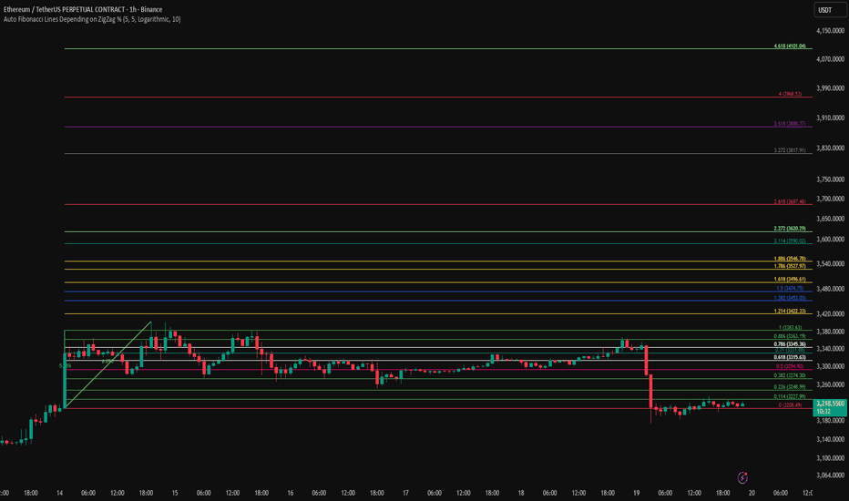
Auto Fibonacci Lines Depending on ZigZag %In the world of technical analysis, few tools are as powerful—or as misused—as Fibonacci Retracements. The Auto Fibonacci Lines Depending on ZigZag % is not just an indicator; it is a complete, automated trading system designed to eliminate subjectivity and bring institutional-grade precision to your charts.
This script automates the identification of significant market structures using a ZigZag algorithm. Once a market swing is mathematically confirmed (based on your deviation settings), it instantly projects a complete suite of Retracement and Extension levels. This allows you to stop guessing where to draw your lines and start focusing on price action.
🧠 The Logic Behind the Indicator
Understanding how your tools work is the first step to trusting them. This script operates on a three-step logic loop:
ZigZag Identification:
The script continuously monitors price action relative to the last known pivot point. It uses a user-defined Deviation % to filter out market noise. A new "Leg" is only confirmed when price reverses by this specific percentage. This ensures that the Fibonacci lines are only drawn on significant market moves, not random chop.
Automated Anchor Points:
Once a downward trend is confirmed (e.g., price drops 30% from the top), the script automatically anchors the Fibonacci tool to the Swing High (Start) and the Swing Low (End). It does this without you needing to click or drag anything.
Dynamic Cleanup:
Markets evolve. A key feature of this script is its self-cleaning mechanism. As soon as a new trend leg is confirmed, the script automatically deletes the old, invalidated Fibonacci lines and draws a fresh set for the new structure. This keeps your chart clean and focused on the now.
🎓 How to Trade This System
This indicator is color-coded to simplify your decision-making process. It moves beyond standard "rainbow" charts by categorizing price levels into three distinct actionable zones.
1. The "Reload Zone" (White Lines: 0.618 - 0.786) ⚪
Role: High-Probability Support / Entry
In institutional trading, the 0.618 (Golden Ratio) to 0.786 region is often where algorithms step in to defend a trend.
Why it works : This is the "discount" area where smart money re-accumulates positions before the next leg up.
2. The "Decision Wall" (Blue Lines: 1.382 - 1.5) 🔵
Role: Strong Resistance / Trend Check
This is a unique feature of this suite. The 1.382 and 1.5 levels often act as a "ceiling" for weak breakouts.
Strategy : If you entered in the White Zone, the Blue Zone is your first major hurdle. If price stalls here, consider securing partial profits.
Warning : A rejection from the Blue Lines often leads to a double-top formation. However, a clean break above the Blue Lines usually signals a parabolic move is beginning.
3. The "Extension Zone" (Yellow, Red, Purple > 1.618) 🟡🔴
Role : Take Profit / Exhaustion
Levels above 1.5 (starting with the 1.618 Golden Extension) are statistical extremes.
Strategy : These are Strict Take Profit levels. Do not FOMO (Fear Of Missing Out) into new long positions here. The probability of a reversal increases drastically as price climbs through these levels (2.618, 3.618, 4.618).
📐 The Mathematical Edge: Logarithmic vs. Linear
One of the most critical features of this script is the ability to toggle between Logarithmic and Linear calculations.
Why use Logarithmic?
If you are trading Crypto (Bitcoin, Altcoins) or high-growth Tech Stocks, linear Fibonacci levels are mathematically incorrect over large moves. A 50% drop from $100 is different than a 50% drop from $10.
This script calculates the percentage difference (Log Scale), ensuring your targets are accurate even during 100%+ parabolic runs.
Why use Linear?
For mature markets like Forex (EURUSD) or Indices (SPX500) where volatility is lower, Linear scaling is the industry standard.
🛠️ Configuration & Best Practices
Deviation % : This is the heartbeat of the indicator.
Swing Trading : Set to 20-30%. This filters out noise and only draws Fibs on major macro moves.
Scalping : Set to 3-5%. This will catch smaller intraday waves.
Text Place : Keeps your chart clean by pushing labels to the right, ensuring they don't overlap with the current price action.
👤 Who Is This Indicator For?
The Disciplined Trader : Who wants to remove emotional bias from their charting.
The Crypto Investor : Who needs accurate Logarithmic targets for long-term holding.
The Confluence Trader : Who combines these automated levels with Order Blocks, RSI, or Volume to find the perfect entry.
⚠️ RISK DISCLAIMER & TERMS OF USE
For Educational Purposes Only:
This script and the strategies described herein are provided strictly for educational and informational purposes. They do not constitute financial, investment, or trading advice. The "Auto Fibonacci Lines" indicator is a tool for technical analysis and should not be used as the sole basis for any trading decision.
No Guarantees:
Past performance of any trading system or methodology is not necessarily indicative of future results. Financial markets are inherently volatile, and trading involves a high level of risk. You could lose some or all of your capital.
User Responsibility:
By using this script, you acknowledge that you are solely responsible for your own trading decisions and risk management. The author assumes no liability for any losses or damages resulting from the use of this tool or the information provided. Always consult with a qualified financial advisor before making investment decisions. インジケーター
LogTrend Retest EngineLogTrend Retest Engine (LTRE)
LogTrend Retest Engine (LTRE) is an advanced trend-continuation overlay designed to identify high-probability breakout retests using logarithmic regression , volatility-adjusted deviation bands , and market regime filtering .
Unlike traditional channels or moving averages, LTRE models price behavior in log space , allowing it to adapt naturally to exponential market moves common in crypto, indices, and long-term trends.
🔹 How It Works
Logarithmic Regression Core
Performs linear regression on log-transformed price and time
Produces a structurally accurate trend midline that scales with price growth
Volatility-Adjusted Deviation Bands
Dynamic upper and lower zones based on statistical deviation
ATR weighting expands or contracts bands as volatility changes
Adaptive Lookback (Optional)
Automatically adjusts regression length using volatility pressure
Faster response in high-volatility environments, smoother in consolidation
🔹 Market Regime Detection
LTRE actively filters conditions using:
R² trend strength (trend quality, not just slope)
Volatility compression vs expansion
User-defined minimum trend strength threshold
Signals are disabled during ranging or low-quality conditions .
🔹 Breakout → Retest Signal Logic
LTRE does not chase breakouts.
Signals trigger only when:
1. Price breaks cleanly outside the deviation band
2. Market regime is confirmed as trending
3. Price performs a controlled retest within a user-defined tolerance
BUY
Break above upper band → retest → trend confirmed
SELL
Break below lower band → retest → trend confirmed
This structure is designed to reduce false breakouts and late entries.
🔹 Visual & Projection Tools
Clean midline and deviation bands
Optional filled zones
Optional future trend projection for forward structure planning
On-chart statistics for trend strength and volatility compression
🔹 Best Use Cases
Trend continuation & pullback strategies
Crypto, Forex, Indices, and equities
Works best on 15m and higher timeframes
⚠️ Disclaimer
LTRE is a decision-support tool , not a complete trading system. Always use proper risk management and confirm signals with additional structure, volume, or higher-timeframe context.
Built for traders who wait for structure — not noise.
インジケーター

Adaptive Log Trend Zones + Retest SignalsAdaptive Log Trend Zones + Retest Signals
Adaptive Log Trend Zones is a trend-following overlay built to identify high-probability breakout retests in strong market conditions. It combines logarithmic regression , volatility-adaptive behavior , and ATR-based trend zones to help traders stay aligned with dominant momentum while avoiding chop.
🔹 Core Features
Logarithmic Regression Midline
Uses linear regression on log price to better handle exponential market moves
Produces smoother, more realistic trend structure on higher timeframes
Volatility-Adaptive Lookback
Automatically expands or contracts the regression length based on ATR volatility
Reacts faster in high volatility, smoother in consolidation
Dynamic Trend Zones
Upper and lower bands are ATR-adjusted and trend-colored
Optional future projection for visual trend guidance
Breakout → Retest Signal Logic
Detects clean breakouts beyond the trend zone
Waits for a controlled pullback (retest) before signaling
Signals only trigger when trend strength is confirmed
Trend Quality Filter
Internal regime detection filters out low-quality, sideways conditions
Uses slope strength and volatility compression to validate entries
🔹 Signals
BUY : Bullish breakout followed by a valid retest in a trending regime
SELL : Bearish breakout followed by a valid retest in a trending regime
Signals are designed for trend continuation , not mean reversion.
🔹 Best Use Cases
Crypto, Forex, and Index markets
Higher timeframes (15m+ recommended)
Trend continuation and pullback strategies
⚠️ Notes
This indicator is not a standalone trading system . Always use proper risk management and confirm signals with structure, volume, or higher-timeframe context.
Designed for traders who prefer structure, patience, and momentum alignment.
インジケーター

LogPressure Envelope [BOSWaves]LogPressure Envelope – Adaptive Volatility & Trend Visualizer
Overview
LogPressure Envelope is a specialized trading tool designed to normalize market behavior using logarithmic price scaling while providing an adaptive framework for volatility and trend detection. The indicator calculates a log-based moving average midline, surrounds it with asymmetric volatility envelopes, and replaces the conventional cloud with progressive fan lines to present price action in a more interpretable form.
By integrating rate-of-change midline coloring, fading trend strength, and structured buy/sell markers, LogPressure Envelope simplifies the reading of complex market dynamics. Its design makes it suitable for multiple trading approaches, including scalping, intraday, and swing trading, where volatility behavior and trend shifts must be understood quickly and objectively.
Unlike static envelope indicators, LogPressure Envelope adapts continuously to price scale and volatility conditions. It evaluates log-transformed prices, applies configurable moving average methods (EMA, SMA, WMA), and derives asymmetric standard-deviation bands for both upside and downside moves. These envelopes are projected as fan lines with adjustable opacity, producing a layered volatility map that evolves with the market.
This system ensures each visual element—midline shading, candle coloring, fan structure, and signal markers—reflects real-time market conditions, allowing traders to interpret volatility expansion, contraction, and directional bias with clarity.
How It Works
The foundation of LogPressure Envelope is the logarithmic transformation of price. By operating in log space, the indicator removes distortions caused by large nominal price differences across assets, enabling consistent analysis of both low-priced and high-priced instruments.
A moving average of log prices is calculated (EMA, SMA, or WMA depending on user input) and then re-converted to normal price scale, forming the log midline. Standard deviation of log prices is then measured over a separate period, with independent multipliers for upside and downside deviations. This asymmetry captures the fact that markets often expand differently in bullish versus bearish phases.
Instead of plotting a filled cloud, the envelope is expressed as ten equidistant fan lines stretching from the lower to upper boundary. Each line is shaded progressively to visualize volatility clustering and directional strength without overloading the chart.
Trend determination is smoothed using a fade mechanism: shifts in bias do not flip instantly but gradually move toward the new state, producing fewer false transitions. Buy and sell markers are generated when trend strength crosses confirmation thresholds, ensuring signals are event-driven and contextually meaningful.
Signals and Visuals
LogPressure Envelope provides multiple layers of structured signals:
Midline Bias – Central moving average colored by rate-of-change, reflecting directional acceleration or deceleration.
Volatility Fan – Ten progressive lines forming a gradient between lower and upper bands, visually encoding volatility spread.
Buy Signals – Labels below bars when upward trend strength is confirmed.
Sell Signals – Labels above bars when downward trend strength is confirmed.
Candle Coloring – Optional shading of candles based on trend alignment with the log midline, highlighting bullish, bearish, or neutral conditions.
These signals remain clear even during high-volatility phases, with visual hierarchy maintained through progressive opacity control.
Interpretation
Trend Analysis : Midline direction and candle coloring provide continuous feedback on prevailing bias. Upward-sloping midlines with blue shading indicate bullish phases, while downward slopes with orange shading confirm bearish conditions.
Volatility and Risk Assessment : Expansion of fan lines indicates rising volatility and potential breakout conditions; contraction indicates consolidation and possible mean reversion.
Signal Confirmation : Buy and sell markers validate transitions when trend strength thresholds are crossed, aligning with volatility envelope dynamics.
Market Context : Asymmetric envelopes allow traders to see where bearish acceleration differs from bullish expansion, improving interpretation of liquidity conditions and institutional pressure.
Strategy Integration
LogPressure Envelope can be applied across trading styles:
Trend Following : Enter trades in the direction of midline bias, confirmed by buy or sell markers.
Pullback Entries : Use midline retests during trending conditions as lower-risk continuation points.
Volatility Breakouts : Identify sharp expansions in fan line spacing as early signals of directional moves.
Reversal Strategies : Fade extreme envelope touches when momentum shows exhaustion and fan contraction begins.
Multi-Timeframe Confirmation : Align signals from higher and lower timeframes to reduce noise and validate trade setups.
Stop-loss levels can be set near the opposite envelope boundary, while targets may be managed through progressive volatility zones or midline convergence.
Advanced Techniques
For greater precision, LogPressure Envelope can be combined with other analytical tools:
Pair with volume or liquidity measures to validate breakout or reversal conditions.
Use momentum indicators to confirm ROC-based midline bias.
Track sequences of fan line expansions and contractions to anticipate regime shifts in volatility.
Apply across multiple timeframes to monitor how volatility clusters align at different market scales.
Adjusting parameters such as envelope multipliers, moving average type, and fade bars allows the indicator to adapt to diverse asset classes and volatility environments.
Inputs and Customization
Midline Type : Select EMA, SMA, or WMA.
Line Opacity : Control visibility of fan lines.
Enable Candle Coloring : Toggle trend-based bar shading.
MA Length / StdDev Length : Define periods for midline and volatility calculation.
Multipliers : Set asymmetric scaling for upside and downside envelopes.
Fade Bars : Control smoothness of trend strength transitions.
Fan Lines : Adjust number of envelope subdivisions for visualization granularity.
Why Use LogPressure Envelope
LogPressure Envelope translates complex volatility and trend interactions into a structured and adaptive framework. By combining logarithmic normalization, asymmetric standard deviation envelopes, and smoothed trend confirmation, it allows traders to:
Normalize price analysis across assets of different scales.
Visualize volatility expansion and contraction in real time.
Identify and confirm directional shifts with objective signal markers.
Apply a disciplined system for trend, breakout, and reversal strategies.
This indicator is designed for traders who want a systematic, visually clear approach to volatility-based market analysis without relying on static bands or arbitrary scaling.
インジケーター

Logarithmic Moving Average (LMA) [QuantAlgo]🟢 Overview
The Logarithmic Moving Average (LMA) uses advanced logarithmic weighting to create a dynamic trend-following indicator that prioritizes recent price action while maintaining statistical significance. Unlike traditional moving averages that use linear or exponential weights, this indicator employs logarithmic decay functions to create a more sophisticated price averaging system that adapts to market volatility and momentum conditions.
The indicator displays a smoothed signal line that oscillates around zero, with positive values indicating bullish momentum and negative values indicating bearish momentum. The signal incorporates trend quality assessment, momentum confirmation, and multiple filtering mechanisms to help traders and investors identify trend continuation and reversal opportunities across different timeframes and asset classes.
🟢 How It Works
The indicator's core innovation lies in its logarithmic weighting system, where weights are calculated using the formula: w = 1.0 / math.pow(math.log(i + steepness), 2) The steepness parameter controls how aggressively recent data is prioritized over historical data, creating a dynamic weight decay that can be fine-tuned for different trading styles. This logarithmic approach provides more nuanced weight distribution compared to exponential moving averages, offering better responsiveness while maintaining stability.
The LMA calculation combines multiple sophisticated components. First, it calculates the logarithmic weighted average of closing prices. Then it measures the slope of this average over a 10-period lookback: lmaSlope = (lma - lma ) / lma * 100 The system also incorporates trend quality assessment using R-squared correlation analysis of log-transformed prices, measuring how well the price data fits a linear trend model over the specified period.
The final signal generation uses the formula: signal = lmaSlope * (0.5 + rSquared * 0.5) which combines the LMA slope with trend quality weighting. When momentum confirmation is enabled, the indicator calculates annualized log-return momentum and applies a multiplier when the momentum direction aligns with the signal direction, strengthening confirmed signals while filtering out weak or counter-trend movements.
🟢 How to Use
1. Signal Interpretation and Threshold Zones
Positive Values (Above Zero): LMA slope indicating bullish momentum with upward price trajectory relative to logarithmic baseline
Negative Values (Below Zero): LMA slope indicating bearish momentum with downward price trajectory relative to logarithmic baseline
Zero Line Crosses: Signal transitions between bullish and bearish regimes, indicating potential trend changes
Long Entry Threshold Zone: Area above positive threshold (default 0.5) indicating confirmed bullish signals suitable for long positions
Short Entry Threshold Zone: Area below negative threshold (default -0.5) indicating confirmed bearish signals suitable for short positions
Extreme Values: Signals exceeding ±1.0 represent strong momentum conditions with higher probability of continuation
2. Momentum Confirmation and Visual Analysis
Signal Color Intensity: Gradient coloring shows signal strength, with brighter colors indicating stronger momentum
Bar Coloring: Optional price bar coloring matches signal direction for quick visual trend identification
Position Labels: Real-time position classification (Bullish/Bearish/Neutral) displayed on the latest bar
Momentum Weight Factor: When short-term log-return momentum aligns with LMA signal direction, the signal receives additional weight confirmation
Trend Quality Component: R-squared values weight the signal strength, with higher correlation indicating more reliable trend conditions
3. Examples: Preconfigured Settings
Default: Universally applicable configuration balanced for medium-term investing and general trading across multiple timeframes and asset classes.
Scalping: Highly responsive setup with shorter period and higher steepness for ultra-short-term trades on 1-15 minute charts, optimized for quick momentum shifts.
Swing Trading: Extended period with moderate steepness and increased smoothing for multi-day positions, designed to filter noise while capturing larger price swings on 1-4 hour and daily charts.
Trend Following: Maximum smoothing with lower steepness for established trend identification, generating fewer but more reliable signals optimal for daily and weekly timeframes.
Mean Reversion: Shorter period with high steepness for counter-trend strategies, more sensitive to extreme moves and reversal opportunities in ranging market conditions.
インジケーター

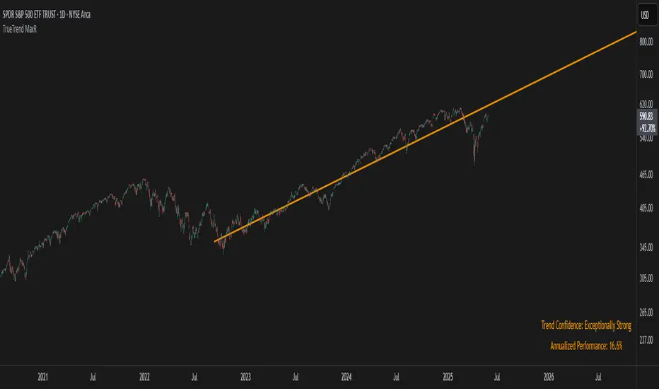
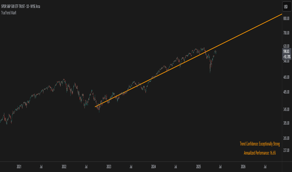
TrueTrend MaxRThe TrueTrend MaxR indicator is designed to identify the most consistent exponential price trend over extended periods. It uses statistical analysis on log-transformed prices to find the trendline that best fits historical price action, and highlights the most frequently tested or traded level within that trend channel.
For optimal results, especially on high timeframes such as weekly or monthly, it is recommended to use this indicator on charts set to logarithmic scale. This ensures proper visual alignment with the exponential nature of long-term price movements.
How it works
The indicator tests 50 different lookback periods, ranging from 300 to 1280 bars. For each period, it:
- Applies a linear regression on the natural logarithm of the price
- Computes the slope and intercept of the trendline
- Calculates the unbiased standard deviation from the regression line
- Measures the correlation strength using Pearson's R coefficient
The period with the highest Pearson R value is selected, meaning the trendline drawn corresponds to the log-scale trend with the best statistical fit.
Trendline and deviation bands
Once the optimal period is identified, the indicator plots:
- A main log-scale trendline
- Upper and lower bands, based on a user-defined multiple of the standard deviation
These bands help visualize how far price deviates from its core trend, and define the range of typical fluctuations.
Point of Control (POC)
Inside the trend channel, the space between upper and lower bands is divided into 15 logarithmic levels. The script evaluates how often price has interacted with each level, using one of two selectable methods:
- Touches: Counts the number of candles crossing each level
- Volume: Weighs each touch by the traded volume at that candle
The level with the highest cumulative interaction is considered the dynamic Point of Control (POC), and is plotted as a line.
Annualized performance and confidence display
When used on daily or weekly timeframes, the script also calculates the annualized return (CAGR) based on the detected trend, and displays:
- A performance estimate in percentage terms
- A textual label describing the confidence level based on the Pearson R value
Why this indicator is useful
- Automatically detects the most statistically consistent exponential trendline
- Designed for log-scale analysis, suited to long-term investment charts
- Highlights key price levels frequently visited or traded within the trend
- Provides objective, data-based trend and volatility insights
- Displays annualized growth rate and correlation strength for quick evaluation
Notes
- All calculations are performed only on the last bar
- No future data is used, and the script does not repaint
- Works on any instrument or timeframe, with optimal use on higher timeframes and logarithmic scaling インジケーター
GIGANEVA V6.61 PublicThis enhanced Fibonacci script for TradingView is a powerful, all-in-one tool that calculates Fibonacci Levels, Fans, Time Pivots, and Golden Pivots on both logarithmic and linear scales. Its ability to compute time pivots via fan intersections and Range interactions, combined with user-friendly features like Bool Fib Right, sets it apart. The script maximizes TradingView’s plotting capabilities, making it a unique and versatile tool for technical analysis across various markets.
1. Overview of the Script
The script appears to be a custom technical analysis tool built for TradingView, improving upon an existing script from TradingView’s Community Scripts. It calculates and plots:
Fibonacci Levels: Standard retracement levels (e.g., 0.236, 0.382, 0.5, 0.618, etc.) based on a user-defined price range.
Fibonacci Fans: Trendlines drawn from a high or low point, radiating at Fibonacci ratios to project potential support/resistance zones.
Time Pivots: Points in time where significant price action is expected, determined by the intersection of Fibonacci Fans or their interaction with key price levels.
Golden Pivots: Specific time pivots calculated when the 0.5 Fibonacci Fan (on a logarithmic or linear scale) intersects with its counterpart.
The script supports both logarithmic and linear price scales, ensuring versatility across different charting preferences. It also includes a feature to extend Fibonacci Fans to the right, regardless of whether the user selects the top or bottom of the range first.
2. Key Components Explained
a) Fibonacci Levels and Fans from Top and Bottom of the "Range"
Fibonacci Levels: These are horizontal lines plotted at standard Fibonacci retracement ratios (e.g., 0.236, 0.382, 0.5, 0.618, etc.) based on a user-defined price range (the "Range"). The Range is typically the distance between a significant high (top) and low (bottom) on the chart.
Example: If the high is $100 and the low is $50, the 0.618 retracement level would be at $80.90 ($50 + 0.618 × $50).
Fibonacci Fans: These are diagonal lines drawn from either the top or bottom of the Range, radiating at Fibonacci ratios (e.g., 0.382, 0.5, 0.618). They project potential dynamic support or resistance zones as price evolves over time.
From Top: Fans drawn downward from the high of the Range.
From Bottom: Fans drawn upward from the low of the Range.
Log and Linear Scale:
Logarithmic Scale: Adjusts price intervals to account for percentage changes, which is useful for assets with large price ranges (e.g., cryptocurrencies or stocks with exponential growth). Fibonacci calculations on a log scale ensure ratios are proportional to percentage moves.
Linear Scale: Uses absolute price differences, suitable for assets with smaller, more stable price ranges.
The script’s ability to plot on both scales makes it adaptable to different markets and user preferences.
b) Time Pivots
Time pivots are points in time where significant price action (e.g., reversals, breakouts) is anticipated. The script calculates these in two ways:
Fans Crossing Each Other:
When two Fibonacci Fans (e.g., one from the top and one from the bottom) intersect, their crossing point represents a potential time pivot. This is because the intersection indicates a convergence of dynamic support/resistance zones, increasing the likelihood of a price reaction.
Example: A 0.618 fan from the top crosses a 0.382 fan from the bottom at a specific bar on the chart, marking that bar as a time pivot.
Fans Crossing Top and Bottom of the Range:
A fan line (e.g., 0.5 fan from the bottom) may intersect the top or bottom price level of the Range at a specific time. This intersection highlights a moment where the fan’s projected support/resistance aligns with a key price level, signaling a potential pivot.
Example: The 0.618 fan from the bottom reaches the top of the Range ($100) at bar 50, marking bar 50 as a time pivot.
c) Golden Pivots
Definition: Golden pivots are a special type of time pivot calculated when the 0.5 Fibonacci Fan on one scale (logarithmic or linear) intersects with the 0.5 fan on the opposite scale (or vice versa).
Significance: The 0.5 level is the midpoint of the Fibonacci sequence and often acts as a critical balance point in price action. When fans at this level cross, it suggests a high-probability moment for a price reversal or significant move.
Example: If the 0.5 fan on a logarithmic scale (drawn from the bottom) crosses the 0.5 fan on a linear scale (drawn from the top) at bar 100, this intersection is labeled a "Golden Pivot" due to its confluence of key Fibonacci levels.
d) Bool Fib Right
This is a user-configurable setting (a boolean input in the script) that extends Fibonacci Fans to the right side of the chart.
Functionality: When enabled, the fans project forward in time, regardless of whether the user selected the top or bottom of the Range first. This ensures consistency in visualization, as the direction of the Range selection (top-to-bottom or bottom-to-top) does not affect the fan’s extension.
Use Case: Traders can use this to project future support/resistance zones without worrying about how they defined the Range, improving usability.
3. Why Is This Code Unique?
Original calculation of Log levels were taken from zekicanozkanli code. Thank you for giving me great Foundation, later modified and applied to Fib fans. The script’s uniqueness stems from its comprehensive integration of Fibonacci-based tools and its optimization for TradingView’s plotting capabilities. Here’s a detailed breakdown:
All-in-One Fibonacci Tool:
Most Fibonacci scripts on TradingView focus on either retracement levels, extensions, or fans.
This script combines:
Fibonacci Levels: Static horizontal lines for retracement and extension.
Fibonacci Fans: Dynamic trendlines for projecting support/resistance.
Time Pivots: Temporal analysis based on fan intersections and Range interactions.
Golden Pivots: Specialized pivots based on 0.5 fan confluences.
By integrating these functions, the script provides a holistic Fibonacci analysis tool, reducing the need for multiple scripts.
Log and Linear Scale Support:
Many Fibonacci tools are designed for linear scales only, which can distort projections for assets with exponential price movements. By supporting both logarithmic and linear scales, the script caters to a wider range of markets (e.g., stocks, forex, crypto) and user preferences.
Time Pivot Calculations:
Calculating time pivots based on fan intersections and Range interactions is a novel feature. Most TradingView scripts focus on price-based Fibonacci levels, not temporal analysis. This adds a predictive element, helping traders anticipate when significant price action might occur.
Golden Pivot Innovation:
The concept of "Golden Pivots" (0.5 fan intersections across scales) is a unique addition. It leverages the symmetry of the 0.5 level and the differences between log and linear scales to identify high-probability pivot points.
Maximized Plot Capabilities:
TradingView imposes limits on the number of plots (lines, labels, etc.) a script can render. This script is coded to fully utilize these limits, ensuring that all Fibonacci levels, fans, pivots, and labels are plotted without exceeding TradingView’s constraints.
This optimization likely involves efficient use of arrays, loops, and conditional plotting to manage resources while delivering a rich visual output.
User-Friendly Features:
The Bool Fib Right option simplifies fan projection, making the tool intuitive even for users who may not consistently select the Range in the same order.
The script’s flexibility in handling top/bottom Range selection enhances usability.
4. Potential Use Cases
Trend Analysis: Traders can use Fibonacci Fans to identify dynamic support/resistance zones in trending markets.
Reversal Trading: Time pivots and Golden Pivots help pinpoint moments for potential price reversals.
Range Trading: Fibonacci Levels provide key price zones for trading within a defined range.
Cross-Market Application: Log/linear scale support makes the script suitable for stocks, forex, commodities, and cryptocurrencies.
The original code was from zekicanozkanli . Thank you for giving me great Foundation. インジケーター

Log Regression Oscillator Channel [BigBeluga]
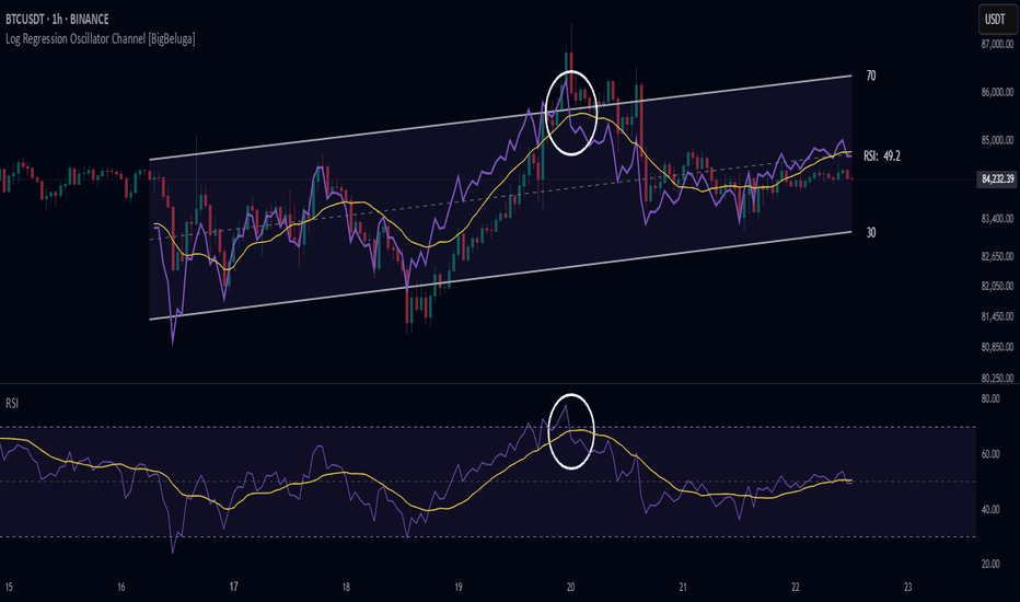
This unique overlay tool blends logarithmic trend analysis with dynamic oscillator behavior. It projects RSI, MFI, or Stochastic lines directly into a log regression channel on the price chart — offering an intuitive way to detect overbought/oversold momentum within the broader price structure.
🔵Key Features:
Logarithmic Regression Channel:
➣ Draws a trend-based channel using logarithmic regression, adapting to price growth curvature over time.
➣ Features upper, lower, and optional midline boundaries to visualize trend flow and range extremes.
Oscillator Overlay (RSI / MFI / Stochastic):
➣ Projects your chosen oscillator inside the channel using dynamic polylines.
➣ Allows switching between RSI, Money Flow Index, or Stochastic for versatile momentum insight.
Threshold-Based Scaling:
➣ The top and bottom of the channel represent traditional oscillator thresholds (e.g., RSI 70/30).
➣ Users can modify the scale in settings to customize what "overbought" or "oversold" means visually.
Signal Line Integration:
➣ Adds a yellow moving average (signal line) for smoother confirmation of oscillator turns.
➣ Helps identify divergence, momentum shifts, and fakeouts with better clarity.
Live Oscillator Readout:
➣ Displays the real-time oscillator value at the right edge of the chart.
➣ Ensures traders stay aware of current momentum levels without switching panels.
🔵Usage:
Momentum Context:
➣ When the oscillator touches the upper regression band, it may signal local overbought pressure.
➣ Touching the lower band may indicate oversold conditions within the current log trend.
Divergence Detection:
➣ Use the oscillator’s behavior relative to the channel slope to spot divergence from price.
➣ For example, RSI rising inside a falling channel can flag early trend shifts.
Trend-Sensitive Entries:
➣ Combine oscillator signals with log channel direction to filter trades in trend alignment.
➣ Signal line crossovers inside the channel act as early warning for momentum turns.
The Log Regression Oscillator Channel transforms how traders view classic momentum tools. By embedding oscillators into a logarithmic trend structure, it offers unmatched clarity on momentum positioning relative to price expansion. Ideal for swing traders, mean-reverters, or trend followers looking to sharpen entries and exits with style. インジケーター
Adaptive Trend FinderAdaptive Trend Finder - The Ultimate Trend Detection Tool
Introducing Adaptive Trend Finder, the next evolution of trend analysis on TradingView. This powerful indicator is an enhanced and refined version of Adaptive Trend Finder (Log), designed to offer even greater flexibility, accuracy, and ease of use.
What’s New?
Unlike the previous version, Adaptive Trend Finder allows users to fully configure and adjust settings directly within the indicator menu, eliminating the need to modify chart settings manually. A major improvement is that users no longer need to adjust the chart's logarithmic scale manually in the chart settings; this can now be done directly within the indicator options, ensuring a smoother and more efficient experience. This makes it easier to switch between linear and logarithmic scaling without disrupting the analysis. This provides a seamless user experience where traders can instantly adapt the indicator to their needs without extra steps.
One of the most significant improvements is the complete code overhaul, which now enables simultaneous visualization of both long-term and short-term trend channels without needing to add the indicator twice. This not only improves workflow efficiency but also enhances chart readability by allowing traders to monitor multiple trend perspectives at once.
The interface has been entirely redesigned for a more intuitive user experience. Menus are now clearer, better structured, and offer more customization options, making it easier than ever to fine-tune the indicator to fit any trading strategy.
Key Features & Benefits
Automatic Trend Period Selection: The indicator dynamically identifies and applies the strongest trend period, ensuring optimal trend detection with no manual adjustments required. By analyzing historical price correlations, it selects the most statistically relevant trend duration automatically.
Dual Channel Display: Traders can view both long-term and short-term trend channels simultaneously, offering a broader perspective of market movements. This feature eliminates the need to apply the indicator twice, reducing screen clutter and improving efficiency.
Fully Adjustable Settings: Users can customize trend detection parameters directly within the indicator settings. No more switching chart settings – everything is accessible in one place.
Trend Strength & Confidence Metrics: The indicator calculates and displays a confidence score for each detected trend using Pearson correlation values. This helps traders gauge the reliability of a given trend before making decisions.
Midline & Channel Transparency Options: Users can fine-tune the visibility of trend channels, adjusting transparency levels to fit their personal charting style without overwhelming the price chart.
Annualized Return Calculation: For daily and weekly timeframes, the indicator provides an estimate of the trend’s performance over a year, helping traders evaluate potential long-term profitability.
Logarithmic Adjustment Support: Adaptive Trend Finder is compatible with both logarithmic and linear charts. Traders who analyze assets like cryptocurrencies, where log scaling is common, can enable this feature to refine trend calculations.
Intuitive & User-Friendly Interface: The updated menu structure is designed for ease of use, allowing quick and efficient modifications to settings, reducing the learning curve for new users.
Why is this the Best Trend Indicator?
Adaptive Trend Finder stands out as one of the most advanced trend analysis tools available on TradingView. Unlike conventional trend indicators, which rely on fixed parameters or lagging signals, Adaptive Trend Finder dynamically adjusts its settings based on real-time market conditions. By combining automatic trend detection, dual-channel visualization, real-time performance metrics, and an intuitive user interface, this indicator offers an unparalleled edge in trend identification and trading decision-making.
Traders no longer have to rely on guesswork or manually tweak settings to identify trends. Adaptive Trend Finder does the heavy lifting, ensuring that users are always working with the strongest and most reliable trends. The ability to simultaneously display both short-term and long-term trends allows for a more comprehensive market overview, making it ideal for scalpers, swing traders, and long-term investors alike.
With its state-of-the-art algorithms, fully customizable interface, and professional-grade accuracy, Adaptive Trend Finder is undoubtedly one of the most powerful trend indicators available.
Try it today and experience the future of trend analysis.
This indicator is a technical analysis tool designed to assist traders in identifying trends. It does not guarantee future performance or profitability. Users should conduct their own research and apply proper risk management before making trading decisions.
// Created by Julien Eche - @Julien_Eche インジケーター

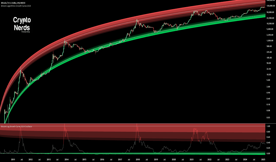
Bitcoin Log Growth Curve OscillatorThis script presents the oscillator version of the Bitcoin Logarithmic Growth Curve 2024 indicator, offering a new perspective on Bitcoin’s long-term price trajectory.
By transforming the original logarithmic growth curve into an oscillator, this version provides a normalized view of price movements within a fixed range, making it easier to identify overbought and oversold conditions.
For a comprehensive explanation of the mathematical derivation, underlying concepts, and overall development of the Bitcoin Logarithmic Growth Curve, we encourage you to explore our primary script, Bitcoin Logarithmic Growth Curve 2024, available here . This foundational script details the regression-based approach used to model Bitcoin’s long-term price evolution.
Normalization Process
The core principle behind this oscillator lies in the normalization of Bitcoin’s price relative to the upper and lower regression boundaries. By applying Min-Max Normalization, we effectively scale the price into a bounded range, facilitating clearer trend analysis. The normalization follows the formula:
normalized price = (upper regresionline − lower regressionline) / (price − lower regressionline)
This transformation ensures that price movements are always mapped within a fixed range, preventing distortions caused by Bitcoin’s exponential long-term growth. Furthermore, this normalization technique has been applied to each of the confidence interval lines, allowing for a structured and systematic approach to analyzing Bitcoin’s historical and projected price behavior.
By representing the logarithmic growth curve in oscillator form, this indicator helps traders and analysts more effectively gauge Bitcoin’s position within its long-term growth trajectory while identifying potential opportunities based on historical price tendencies. インジケーター
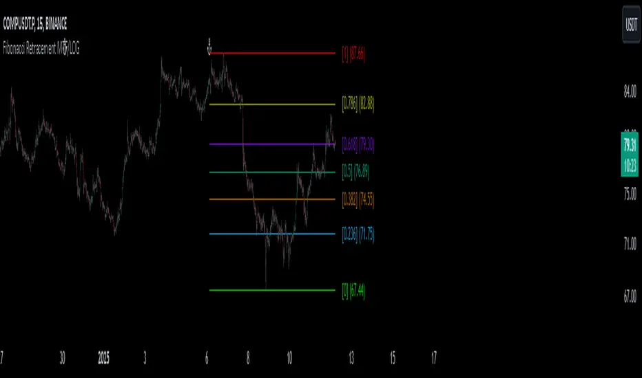
Fibonacci Retracement MTF/LOGIn Pine Script, there’s always a shorter way to achieve a result. As far as I can see, there isn’t an indicator among the community scripts that can produce Fibonacci Retracement levels (linear and logarithmic) as multiple time frame results based on a reference 🍺 This script, which I developed a long time ago, might serve as a starting point to fill this gap.
OVERVIEW
This indicator is a short and simple script designed to display Fibonacci Retracement levels on the chart according to user preferences, aiming to build the structure of support and resistance.
ORIGINALITY
This script:
Can calculate 'retracement' results from higher time frames.
Can recall previous time frame results using its reference parameter.
Performs calculations based on both linear and logarithmic scales.
Offers optional multipliers and appearance settings to simplify users’ tasks
CONCEPTS
Fibonacci Retracement is a technical analysis tool used to predict potential reversal points in an asset's price after a significant movement. This indicator identifies possible support and resistance levels by measuring price movements between specific points in a trend, using certain ratios derived from the Fibonacci sequence. It is based on impulsive price actions.
MECHANICS
This indicator first identifies the highest and lowest prices in the time frame specified by the user. Next, it determines the priority order of the bars where these prices occurred. Finally, it defines the trend direction. Once the trend direction is determined, the "Retracement" levels are constructed.
FUNCTIONS
The script contains two functions:
f_ret(): Generates levels based on the multiplier parameter.
f_print(): Handles the visualization by drawing the levels on the chart and positioning the labels in alignment with the levels. It utilizes parameters such as ordinate, confirmation, multiplier, and color for customization
NOTES
The starting bar for the time frame entered by the user must exist on the chart. Otherwise, the trend direction cannot be determined correctly, and the levels may be drawn inaccurately. This is also mentioned in the tooltip of the TimeFrame parameter.
I hope it helps everyone. Do not forget to manage your risk. And trade as safely as possible. Best of luck! インジケーター

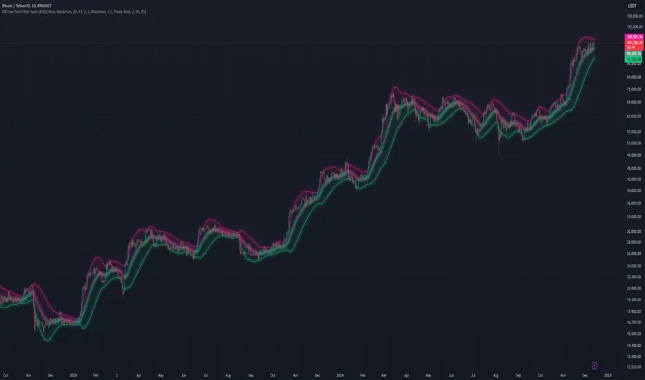
FIR Low Pass Filter Suite (FIR)The FIR Low Pass Filter Suite is an advanced signal processing indicator that applies finite impulse response (FIR) filtering techniques to price data. At its core, the indicator uses windowed-sinc filtering, which provides optimal frequency response characteristics for separating trend from noise in financial data.
The indicator offers multiple window functions including Kaiser, Kaiser-Bessel Derived (KBD), Hann, Hamming, Blackman, Triangular, and Lanczos. Each window type provides different trade-offs between main-lobe width and side-lobe attenuation, allowing users to fine-tune the frequency response characteristics of the filter. The Kaiser and KBD windows provide additional control through an alpha parameter that adjusts the shape of the window function.
A key feature is the ability to operate in either linear or logarithmic space. Logarithmic filtering can be particularly appropriate for financial data due to the multiplicative nature of price movements. The indicator includes an envelope system that can adaptively calculate bands around the filtered price using either arithmetic or geometric deviation, with separate controls for upper and lower bands to account for the asymmetric nature of market movements.
The implementation handles edge effects through proper initialization and offers both centered and forward-only filtering modes. Centered mode provides zero phase distortion but introduces lag, while forward-only mode operates causally with no lag but introduces some phase distortion. All calculations are performed using vectorized operations for efficiency, with carefully designed state management to handle the filter's warm-up period.
Visual feedback is provided through customizable color gradients that can reflect the current trend direction, with optional glow effects and background fills to enhance visibility. The indicator maintains high numerical precision throughout its calculations while providing smooth, artifact-free output suitable for both analysis and visualization.
インジケーター

Logarithmic Regression AlternativeLogarithmic regression is typically used to model situations where growth or decay accelerates rapidly at first and then slows over time. Bitcoin is a good example.
𝑦 = 𝑎 + 𝑏 * ln(𝑥)
With this logarithmic regression (log reg) formula 𝑦 (price) is calculated with constants 𝑎 and 𝑏, where 𝑥 is the bar_index .
Instead of using the sum of log x/y values, together with the dot product of log x/y and the sum of the square of log x-values, to calculate a and b, I wanted to see if it was possible to calculate a and b differently.
In this script, the log reg is calculated with several different assumed a & b values, after which the log reg level is compared to each Swing. The log reg, where all swings on average are closest to the level, produces the final 𝑎 & 𝑏 values used to display the levels.
🔶 USAGE
The script shows the calculated logarithmic regression value from historical swings, provided there are enough swings, the price pattern fits the log reg model, and previous swings are close to the calculated Top/Bottom levels.
When the price approaches one of the calculated Top or Bottom levels, these levels could act as potential cycle Top or Bottom.
Since the logarithmic regression depends on swing values, each new value will change the calculation. A well-fitted model could not fit anymore in the future.
Swings are based on Weekly bars. A Top Swing, for example, with Swing setting 30, is the highest value in 60 weeks. Thirty bars at the left and right of the Swing will be lower than the Top Swing. This means that a confirmation is triggered 30 weeks after the Swing. The period will be automatically multiplied by 7 on the daily chart, where 30 becomes 210 bars.
Please note that the goal of this script is not to show swings rapidly; it is meant to show the potential next cycle's Top/Bottom levels.
🔹 Multiple Levels
The script includes the option to display 3 Top/Bottom levels, which uses different values for the swing calculations.
Top: 'high', 'maximum open/close' or 'close'
Bottom: 'low', 'minimum open/close' or 'close'
These levels can be adjusted up/down with a percentage.
Lastly, an "Average" is included for each set, which will only be visible when "AVG" is enabled, together with both Top and Bottom levels.
🔹 Notes
Users have to check the validity of swings; the above example only uses 1 Top Swing for its calculations, making the Top level unreliable.
Here, 1 of the Bottom Swings is pretty far from the bottom level, changing the swing settings can give a more reliable bottom level where all swings are close to that level.
Note the display was set at "Logarithmic", it can just as well be shown as "Regular"
In the example below, the price evolution does not fit the logarithmic regression model, where growth should accelerate rapidly at first and then slows over time.
Please note that this script can only be used on a daily timeframe or higher; using it at a lower timeframe will show a warning. Also, it doesn't work with bar-replay.
🔶 DETAILS
The code gathers data from historical swings. At the last bar, all swings are calculated with different a and b values. The a and b values which results in the smallest difference between all swings and Top/Bottom levels become the final a and b values.
The ranges of a and b are between -20.000 to +20.000, which means a and b will have the values -20.000, -19.999, -19.998, -19.997, -19.996, ... -> +20.000.
As you can imagine, the number of calculations is enormous. Therefore, the calculation is split into parts, first very roughly and then very fine.
The first calculations are done between -20 and +20 (-20, -19, -18, ...), resulting in, for example, 4.
The next set of calculations is performed only around the previous result, in this case between 3 (4-1) and 5 (4+1), resulting in, for example, 3.9. The next set goes even more in detail, for example, between 3.8 (3.9-0.1) and 4.0 (3.9 + 0.1), and so on.
1) -20 -> +20 , then loop with step 1 (result (example): 4 )
2) 4 - 1 -> 4 +1 , then loop with step 0.1 (result (example): 3.9 )
3) 3.9 - 0.1 -> 3.9 +0.1 , then loop with step 0.01 (result (example): 3.93 )
4) 3.93 - 0.01 -> 3.93 +0.01, then loop with step 0.001 (result (example): 3.928)
This ensures complicated calculations with less effort.
These calculations are done at the last bar, where the levels are displayed, which means you can see different results when a new swing is found.
Also, note that this indicator has been developed for a daily (or higher) timeframe chart.
🔶 SETTINGS
Three sets
High/Low
• color setting
• Swing Length settings for 'High' & 'Low'
• % adjustment for 'High' & 'Low'
• AVG: shows average (when both 'High' and 'Low' are enabled)
Max/Min (maximum open/close, minimum open/close)
• color setting
• Swing Length settings for 'Max' & 'Min'
• % adjustment for 'Max' & 'Min'
• AVG: shows average (when both 'Max' and 'Min' are enabled)
Close H/Close L (close Top/Bottom level)
• color setting
• Swing Length settings for 'Close H' & 'Close L'
• % adjustment for 'Close H' & 'Close L'
• AVG: shows average (when both 'Close H' and 'Close L' are enabled)
Show Dashboard, including Top/Bottom levels of the desired source and calculated a and b values.
Show Swings + Dot size
インジケーター

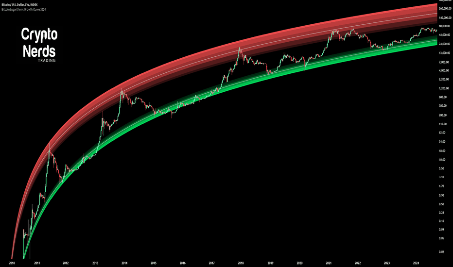
Bitcoin Logarithmic Growth Curve 2024The Bitcoin logarithmic growth curve is a concept used to analyze Bitcoin's price movements over time. The idea is based on the observation that Bitcoin's price tends to grow exponentially, particularly during bull markets. It attempts to give a long-term perspective on the Bitcoin price movements.
The curve includes an upper and lower band. These bands often represent zones where Bitcoin's price is overextended (upper band) or undervalued (lower band) relative to its historical growth trajectory. When the price touches or exceeds the upper band, it may indicate a speculative bubble, while prices near the lower band may suggest a buying opportunity.
Unlike most Bitcoin growth curve indicators, this one includes a logarithmic growth curve optimized using the latest 2024 price data, making it, in our view, superior to previous models. Additionally, it features statistical confidence intervals derived from linear regression, compatible across all timeframes, and extrapolates the data far into the future. Finally, this model allows users the flexibility to manually adjust the function parameters to suit their preferences.
The Bitcoin logarithmic growth curve has the following function:
y = 10^(a * log10(x) - b)
In the context of this formula, the y value represents the Bitcoin price, while the x value corresponds to the time, specifically indicated by the weekly bar number on the chart.
How is it made (You can skip this section if you’re not a fan of math):
To optimize the fit of this function and determine the optimal values of a and b, the previous weekly cycle peak values were analyzed. The corresponding x and y values were recorded as follows:
113, 18.55
240, 1004.42
451, 19128.27
655, 65502.47
The same process was applied to the bear market low values:
103, 2.48
267, 211.03
471, 3192.87
676, 16255.15
Next, these values were converted to their linear form by applying the base-10 logarithm. This transformation allows the function to be expressed in a linear state: y = a * x − b. This step is essential for enabling linear regression on these values.
For the cycle peak (x,y) values:
2.053, 1.268
2.380, 3.002
2.654, 4.282
2.816, 4.816
And for the bear market low (x,y) values:
2.013, 0.394
2.427, 2.324
2.673, 3.504
2.830, 4.211
Next, linear regression was performed on both these datasets. (Numerous tools are available online for linear regression calculations, making manual computations unnecessary).
Linear regression is a method used to find a straight line that best represents the relationship between two variables. It looks at how changes in one variable affect another and tries to predict values based on that relationship.
The goal is to minimize the differences between the actual data points and the points predicted by the line. Essentially, it aims to optimize for the highest R-Square value.
Below are the results:
It is important to note that both the slope (a-value) and the y-intercept (b-value) have associated standard errors. These standard errors can be used to calculate confidence intervals by multiplying them by the t-values (two degrees of freedom) from the linear regression.
These t-values can be found in a t-distribution table. For the top cycle confidence intervals, we used t10% (0.133), t25% (0.323), and t33% (0.414). For the bottom cycle confidence intervals, the t-values used were t10% (0.133), t25% (0.323), t33% (0.414), t50% (0.765), and t67% (1.063).
The final bull cycle function is:
y = 10^(4.058 ± 0.133 * log10(x) – 6.44 ± 0.324)
The final bear cycle function is:
y = 10^(4.684 ± 0.025 * log10(x) – -9.034 ± 0.063)
The main Criticisms of growth curve models:
The Bitcoin logarithmic growth curve model faces several general criticisms that we’d like to highlight briefly. The most significant, in our view, is its heavy reliance on past price data, which may not accurately forecast future trends. For instance, previous growth curve models from 2020 on TradingView were overly optimistic in predicting the last cycle’s peak.
This is why we aimed to present our process for deriving the final functions in a transparent, step-by-step scientific manner, including statistical confidence intervals. It's important to note that the bull cycle function is less reliable than the bear cycle function, as the top band is significantly wider than the bottom band.
Even so, we still believe that the Bitcoin logarithmic growth curve presented in this script is overly optimistic since it goes parly against the concept of diminishing returns which we discussed in this post:
This is why we also propose alternative parameter settings that align more closely with the theory of diminishing returns.
Our recommendations:
Drawing on the concept of diminishing returns, we propose alternative settings for this model that we believe provide a more realistic forecast aligned with this theory. The adjusted parameters apply only to the top band: a-value: 3.637 ± 0.2343 and b-parameter: -5.369 ± 0.6264. However, please note that these values are highly subjective, and you should be aware of the model's limitations.
Conservative bull cycle model:
y = 10^(3.637 ± 0.2343 * log10(x) - 5.369 ± 0.6264)
インジケーター
E9 PLRRThe E9 PLRR (Power Law Residual Ratio) is a custom-built indicator designed to evaluate the overvaluation or undervaluation of an asset, specifically by utilizing logarithmic price data and a power law-based model. It leverages a dynamic regression technique to assess the deviation of the current price from its expected value, giving insights into how much the price deviates from its long-term trend.
This indicator is primarily used to detect market extremes and cycles, often used in the analysis of long-term price movements in assets like Bitcoin, where cyclical behavior and significant price deviations are common.
This chart is back from 2019 and shows (From left to right) 2018 Bear market bottom at $3.5k (Dark Blue) , following a peak at 12k (dark red) before the Covid crash back down to EUROTLX:4K (Dark blue)
Key Components
Logarithmic Price Data:
The indicator works with logarithmic price data (ohlc4), which represents the average of open, high, low, and close prices. The logarithmic transformation is crucial in financial modeling, especially when analyzing long-term price data, as it normalizes exponential price growth patterns.
Dynamic Exponent 𝑘:
The model calculates a dynamic exponent k using regression, which defines the power law relationship between time and price. This exponent is essential in determining the expected power law price return and how far the current price deviates from that expected trend.
Power Law Price Return:
The power law price return is computed using the dynamic exponent
k over a defined period, such as 365 days (1 year). It represents the theoretical price return based on a power law relationship, which is used to compare against the actual logarithmic price data.
Risk-Free Rate:
The indicator incorporates an adjustable risk-free rate, allowing users to model the opportunity cost of holding an asset compared to risk-free alternatives. By default, the risk-free rate is set to 0%, but this can be modified depending on the user's requirements.
Volatility Adjustment:
A key feature of the PLRR is its ability to adjust for price volatility. The indicator smooths out short-term price fluctuations using a moving average, helping to detect longer-term cycles and trends.
PLRR Calculation:
The core of the indicator is the calculation of the Power Law Residual Ratio (PLRR). This is derived by subtracting the expected power law price return and risk-free rate from the logarithmic price return, then multiplying the result by a user-defined multiplier.
Color Gradient:
The PLRR values are represented visually using a color gradient. This gradient helps the user quickly identify whether the asset is in an undervalued, fair value, or overvalued state:
Dark Blue to Light Blue: Indicates undervaluation, with increasing blue tones representing a higher degree of undervaluation.
Green to Yellow: Represents fair value, where the price is aligned with the expected power law return.
Orange to Dark Red: Indicates overvaluation, with increasing red tones representing a higher degree of overvaluation.
Zero Line:
A zero line is plotted on the indicator chart, serving as a reference point. Values above the zero line suggest potential overvaluation, while values below indicate potential undervaluation.
Dots Visualization:
The PLRR is plotted using dots, with each dot color-coded based on the PLRR value. This dot-based visualization makes it easier to spot significant changes or reversals in market sentiment without overwhelming the user with continuous lines.
Bar Coloring:
The chart’s bars are colored in accordance with the PLRR value at each point in time, making it visually clear when an asset is potentially overvalued or undervalued.
Indicator Functionality
Cycle Identification : The E9 PLRR is especially useful for identifying cyclical market behavior. In assets like Bitcoin, which are known for their boom-bust cycles, the PLRR can help pinpoint when the market is likely entering a peak (overvaluation) or a trough (undervaluation).
Overvaluation and Undervaluation Detection: By comparing the current price to its expected power law return, the PLRR helps traders assess whether an asset is trading above or below its fair value. This is critical for long-term investors seeking to enter the market at undervalued levels and exit during periods of overvaluation.
Trend Following: The indicator helps users identify the broader trend by smoothing out short-term volatility. This makes it useful for both momentum traders looking to ride trends and contrarian traders seeking to capitalize on market extremes.
Customization
The E9 PLRR allows users to fine-tune several parameters based on their preferences or specific market conditions:
Lookback Period:
The user can adjust the lookback period (default: 100) to modify how the moving average and regression are calculated.
Risk-Free Rate:
Adjusting the risk-free rate allows for more realistic modeling of the opportunity cost of holding the asset.
Multiplier:
The multiplier (default: 5.688) amplifies the sensitivity of the PLRR, allowing users to adjust how aggressively the indicator responds to price movements.
This indicator was inspired by the works of Ashwin & PlanG and their work around powerLaw. Thank you. I hall be working on the calculation of this indicator moving forward to make improvements and optomisations. インジケーター

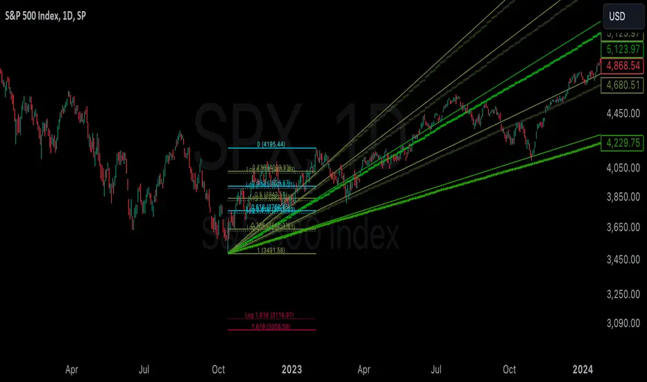
Linear and Logarithmic Fibonacci Levels and (Price&Time) FansIntroduction
The Fibonacci Retracement tool is a go-to for traders looking to spot potential support and resistance levels. By measuring the distance between swing highs and lows, you can apply Fibonacci ratios like 0.236, 0.382, and 0.618 to predict key market levels.
Traditionally, these levels are set by dividing this distance into equal parts—known as Linear Levels. A more refined approach, Logarithmic Price and Time Levels, divides the distance into proportionally equal segments. Plus, this indicator now includes Fibonacci fans, adding another layer of analysis by projecting potential price levels using trendlines based on Fibonacci ratios.
This tool makes it easier to identify both Linear and Logarithmic levels while also leveraging Fibonacci fans for a more complete market view.
Applications
Logarithmic Levels and Fibonacci fans are ideal for volatile markets. In crypto, they’re especially effective for BTCUSDT (check out the wick from January 23, 2024). They also help spot accumulation and distribution patterns in high-volume altcoins like FETUSDT . In traditional markets, they’re useful for tracking stocks like TSLA and NVDA with extreme price swings, as well as indices in inflation-affected markets like XU100 , or recession-hit currency pairs like JPYUSD .
How to Use
This indicator is intuitive and similar to TradingView’s Fibonacci Tool. Select your reference levels (Level 1 and Level 0), then tweak the settings to customize your analysis, including adding Fibonacci fans for extra insights.
Why It’s Different
Unlike TradingView’s tool, which forces you to switch to a logarithmic scale (messing with other indicators and trend lines), this indicator lets you view both Linear and Logarithmic levels—and Fibonacci fans on Price and Time Series—without changing your chart’s scale. The original Fibonacci Code was derived from zekicanozkanli, modified and upgraded to plot fib front and back fans as well. Due to TV Max Plot restrictions I need to publish just Front and Back and Front Fibs separately. インジケーター
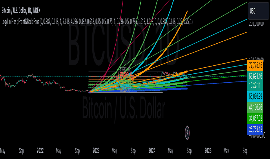
Linear and Logarithmic Fibonacci Levels and FansIntroduction
The Fibonacci Retracement tool is a go-to for traders looking to spot potential support and resistance levels. By measuring the distance between swing highs and lows, you can apply Fibonacci ratios like 0.236, 0.382, and 0.618 to predict key market levels.
Traditionally, these levels are set by dividing this distance into equal parts—known as Linear Levels. A more refined approach, Logarithmic Levels, divides the distance into proportionally equal segments. Plus, this indicator now includes Fibonacci fans, adding another layer of analysis by projecting potential price levels using trendlines based on Fibonacci ratios.
This tool makes it easier to identify both Linear and Logarithmic levels while also leveraging Fibonacci fans for a more complete market view.
Applications
Logarithmic Levels and Fibonacci fans are ideal for volatile markets. In crypto, they’re especially effective for BTCUSDT (check out the wick from January 23, 2024). They also help spot accumulation and distribution patterns in high-volume altcoins like FETUSDT . In traditional markets, they’re useful for tracking stocks like TSLA and NVDA with extreme price swings, as well as indices in inflation-affected markets like XU100 , or recession-hit currency pairs like JPYUSD .
How to Use
This indicator is intuitive and similar to TradingView’s Fibonacci Tool. Select your reference levels (Level 1 and Level 0), then tweak the settings to customize your analysis, including adding Fibonacci fans for extra insights.
Why It’s Different
Unlike TradingView’s tool, which forces you to switch to a logarithmic scale (messing with other indicators and trend lines), this indicator lets you view both Linear and Logarithmic levels—and Fibonacci fans—without changing your chart’s scale. The original Fibonacci Code was derived from zekicanozkanli, modified and upgraded to plot fib fans as well. インジケーター

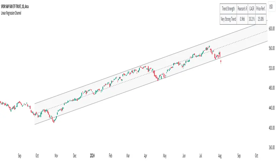
Linear Regression ChannelLinear Regression Channel with Logarithmic Scale Option
This advanced Linear Regression Channel indicator offers traders a powerful tool for technical analysis, with unique features that set it apart from standard implementations.
Key Features:
Logarithmic Scale Option: One of the most distinctive aspects of this indicator is the ability to switch between classic and logarithmic scales. This feature is particularly valuable for long-term analysis, as it ensures that equal percentage changes are represented equally, regardless of the price level.
Flexible Start Date: Unlike many indicators that rely on a fixed number of periods, this tool allows users to set a specific start date and time. This feature provides precise control over the regression analysis timeframe, enhancing its adaptability to various trading strategies.
Customizable Channel Settings: Users can adjust the upper and lower deviation multipliers, allowing for fine-tuning of the channel width to suit different market conditions and trading styles.
Trend Strength Indicator: An optional feature that displays the strength of the trend based on the Pearson correlation coefficient, offering additional insight into the reliability of the current trend.
Comprehensive Visual Customization: The indicator offers extensive color and style options for the regression line, upper and lower channel lines, and fill areas, allowing traders to create a visually appealing and easy-to-read chart setup.
Extended Line Options: Users can choose to extend the regression lines to the left, right, or both, facilitating projection and analysis of future price movements.
Multiple Alert Conditions: The indicator includes four alert conditions for crossing the upper deviation, lower deviation, and the main regression line in both directions, enhancing its utility for active traders.
Why Choose This Indicator:
The combination of logarithmic scale option and flexible start date setting makes this Linear Regression Channel uniquely suited for both short-term and long-term analysis. The logarithmic scale is particularly beneficial for analyzing assets with significant price changes over time, as it normalizes percentage moves across different price levels. This feature, coupled with the ability to set a precise start date, allows traders to perform more accurate and relevant regression analyses, especially when studying specific market cycles or events.
Moreover, the trend strength indicator and customizable visual elements provide traders with a comprehensive tool that not only identifies potential support and resistance levels but also offers insight into the reliability and strength of the current trend.
In summary, this Linear Regression Channel indicator combines flexibility, precision, and insightful analytics, making it an invaluable tool for traders seeking to enhance their technical analysis capabilities on TradingView. インジケーター

インジケーター