インジケーター

ストラテジー

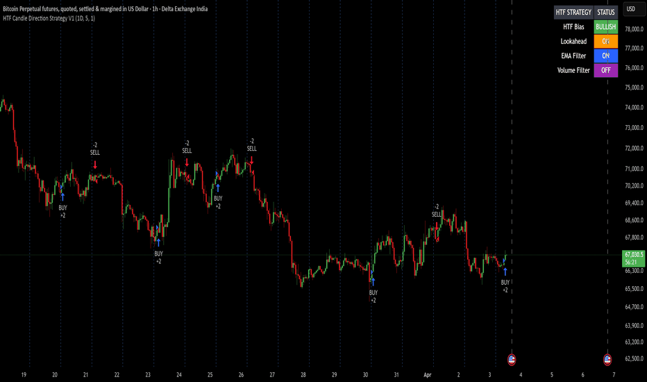
HTF Candle Direction Strategy V1🔹 Title
HTF Candle Direction Strategy V1
🔹 Short Description
Higher Timeframe (HTF) bias-based strategy with optional EMA & volume filters and controlled daily execution.
🔹 Full Description
📌 Overview
HTF Candle Direction Strategy V1 is a simple yet powerful trend-following strategy that trades in the direction of a selected Higher Timeframe (HTF) candle.
The core idea is straightforward:
If the HTF candle is bullish → look for BUY trades
If the HTF candle is bearish → look for SELL trades
This helps traders align with the broader market trend while executing trades on lower timeframes.
⚙️ How It Works
The script fetches HTF Open and Close prices
Determines directional bias:
Bullish Bias → HTF Close > HTF Open
Bearish Bias → HTF Close < HTF Open
Trades are executed only when:
Signals are enabled
Selected direction (Buy/Sell) is enabled
Filters (if enabled) are satisfied
Only one trade per day is allowed
🔍 Features
✅ Higher Timeframe Bias Trading
Trade in alignment with HTF trend
Works on any timeframe combination
✅ Lookahead Mode (Backtesting vs Real Trading)
ON → Faster signals but repaints
OFF → Realistic, non-repainting behavior
✅ EMA Filter (Optional)
Confirms trend using EMA
Buy only above EMA
Sell only below EMA
✅ Volume Filter (Optional)
Trades only when volume is strong
Helps avoid weak market conditions
✅ One Trade Per Day Logic
Prevents overtrading
Keeps strategy disciplined
✅ Built-in Alerts
BUY & SELL alerts included
Ready for automation
✅ Live Dashboard
Displays:
HTF Bias
Lookahead status
EMA filter status
Volume filter status
📊 Dashboard Information
The dashboard (top-right) provides real-time status:
HTF Bias → Current market direction
Lookahead → ON (Repainting) / OFF (Safe)
EMA Filter → Enabled / Disabled
Volume Filter → Enabled / Disabled
⚠️ Important Notes
Lookahead ON = Repainting
Use only for backtesting or analysis
For real trading, always use:
👉 Lookahead OFF
Strategy takes only one trade per day, so performance depends on HTF accuracy
🎯 Best Use Cases
Intraday trading with HTF confirmation
Trend-following strategies
Index, Forex, Crypto markets
Scalping with higher timeframe bias
💡 Recommended Settings
HTF: 4H / Daily
EMA: 50 or 200
Lookahead: OFF (for live trading)
Volume Filter: Optional
🔔 Alerts
BUY Signal → HTF Bullish + filters satisfied
SELL Signal → HTF Bearish + filters satisfied
🚀 Final Notes
This strategy is designed for simplicity, clarity, and disciplined execution.
It avoids overtrading and focuses on high-probability directional setups.
⚠️ Disclaimer
This script is provided for educational and informational purposes only and should not be considered financial advice.
Trading in financial markets involves significant risk, and you may lose all or part of your capital. Past performance of this strategy does not guarantee future results.
This strategy uses higher timeframe data and optional lookahead logic. When lookahead is enabled, signals may repaint, meaning results shown on historical data may differ from real-time performance.
Users are strongly advised to:
Test the strategy on demo accounts before using real capital
Use proper risk management
Understand how the strategy works before trading
The author is not responsible for any financial losses or damages resulting from the use of this script. ストラテジー
Probability Live Table (Juan)The Probability Table Live is an advanced indicator for TradingView designed to display real-time probabilities of price movement for any currency pair and timeframe. This tool organizes the information into a clear and visual table, using intuitive colors to quickly interpret trend strength and the likelihood of continuation or retracement.
🔹 What the chart includes:
Mode → Indicates the current trend: UPTREND or DOWNTREND
Continuation Rate (Cont. Rate) → Probability that the trend will continue strong (30–95%)
Probability Retest → Probability that the price will safely retrace to the key zone (EMA50), adjusted for momentum and distance
Valid Lows / Valid Highs → Count of reliable recent swings (max. 100)
Breakout → Number of confirmed recent breakouts, filtered by strength and relevance
Streak → Streak of candles in the direction of the trend, shown as a %
BOS / CHOCH → Signals for Break of Structure and Change of Character, with dynamic probability
🌈 Dynamic colors: Green → strong and favorable conditions Yellow → medium conditions Red → weak or cautionary conditions Light Blue → recent swings and breakouts 💡 Advantages: Live bar-by-bar predictions. Real and dynamic probabilities for quick decision-making. Compatible with any pair and timeframe. Ideal for fund traders, swing traders, and day traders. With this chart, you can see at a glance the strength of the trend, the probability of continuation or retracement, and market structure signals, all in a single, easy-to-read visual panel. インジケーター

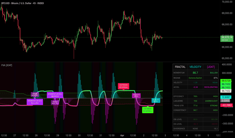
Fractal Velocity Accelerator [JOAT]Fractal Velocity Accelerator
Introduction
The Fractal Velocity Accelerator is an advanced open-source momentum indicator that combines fractal efficiency measurement, adaptive Laguerre filtering, and Gaussian smoothing to create a multi-dimensional momentum oscillator with institutional-grade signal generation. This indicator transforms raw price data into a sophisticated momentum measurement system that reveals not just momentum direction and strength, but also velocity, acceleration, and regime characteristics.
Unlike traditional momentum indicators that simply measure rate of change, this system analyzes the efficiency of price movement through fractal mathematics, applies adaptive lag reduction through Laguerre transforms, and smooths data using 4th-order Gauss filters. The result is a momentum oscillator that responds quickly to genuine momentum shifts while filtering out noise and false signals.
Why This Indicator Exists
This indicator addresses fundamental limitations in traditional momentum analysis by introducing fractal efficiency concepts and adaptive filtering:
4th-Order Gauss Filter: Ultra-smooth OHLC data processing that eliminates noise while preserving genuine price movements
Fractal Efficiency Engine: Logarithmic path efficiency measurement that quantifies how directly price moves from point A to point B
Adaptive Laguerre Transform: Dynamic lag reduction that adjusts based on fractal efficiency, responding faster during efficient moves
Percentile-Based Bands: Self-adjusting overbought/oversold zones that adapt to each instrument's unique momentum characteristics
Velocity and Acceleration Tracking: First and second derivative calculations that identify momentum shifts before they're obvious
Momentum Regime Classification: Seven-level regime system from Extreme Bearish to Extreme Bullish with confidence measurements
Divergence Detection: Fractal-based divergence scanner that identifies price-momentum asymmetries
Each component provides unique intelligence about momentum dynamics. Gauss filtering ensures clean data, fractal efficiency measures directional clarity, Laguerre adaptation reduces lag, percentile bands provide context, velocity/acceleration track changes, regime classification guides strategy, and divergences reveal hidden shifts.
Core Components Explained
1. 4th-Order Gauss Filter System
The indicator applies a sophisticated Gaussian filter to all OHLC data:
w = (2.0 * math.pi / gaussLength)
beta = (1 - math.cos(w)) / (math.pow(1.414, 2.0 / betaDev) - 1)
alpha = (-beta + math.sqrt(beta * beta + 2 * beta))
Gc := math.pow(alpha, 4) * close +
4 * (1.0 - alpha) * nz(Gc ) -
6 * math.pow(1 - alpha, 2) * nz(Gc ) +
4 * math.pow(1 - alpha, 3) * nz(Gc ) -
math.pow(1 - alpha, 4) * nz(Gc )
This 4th-order filter provides exceptional smoothing while maintaining responsiveness. The filter uses four previous values with specific weightings that create a bell curve response, eliminating high-frequency noise while preserving genuine price movements.
The beta deviation parameter (default 2.0) controls filter aggressiveness. Higher values create more smoothing but add lag. Lower values maintain responsiveness but allow more noise. The default balances these tradeoffs optimally for most instruments.
2. Fractal Efficiency Calculation
Fractal efficiency measures how efficiently price moves by comparing net displacement to total path length:
sumRange = math.sum((math.max(Gh, nz(Gc )) - math.min(Gl, nz(Gc ))), fractalLength)
totalRange = ta.highest(Gh, fractalLength) - ta.lowest(Gl, fractalLength)
fractalGamma = if totalRange > 0
math.log(sumRange / totalRange) / math.log(fractalLength)
else
0.0
fractalEfficiency = math.max(0, math.min(1, (fractalGamma + 1) / 2))
The calculation uses logarithmic scaling to measure path complexity. When price moves in a straight line (high efficiency), the ratio approaches 1.0. When price moves erratically (low efficiency), the ratio approaches 0.0.
Fractal efficiency is normalized to 0-1 range where:
- 1.0 = Perfect efficiency (straight line movement)
- 0.7-1.0 = High efficiency (strong trending)
- 0.4-0.7 = Moderate efficiency (developing trend)
- 0.0-0.4 = Low efficiency (choppy/ranging)
This measurement is crucial because it determines how aggressively the Laguerre filter adapts.
3. Adaptive Laguerre Transform
The Laguerre filter applies adaptive lag reduction based on fractal efficiency:
gamma = laguerreGamma * (1 - fractalEfficiency) + 0.1 * fractalEfficiency
L0 := (1 - gamma) * Gc + gamma * nz(L0 )
L1 := -gamma * L0 + nz(L0 ) + gamma * nz(L1 )
L2 := -gamma * L1 + nz(L1 ) + gamma * nz(L2 )
L3 := -gamma * L2 + nz(L2 ) + gamma * nz(L3 )
cu = (L0 > L1 ? L0 - L1 : 0) + (L1 > L2 ? L1 - L2 : 0) + (L2 > L3 ? L2 - L3 : 0)
cd = (L0 < L1 ? L1 - L0 : 0) + (L1 < L2 ? L2 - L1 : 0) + (L2 < L3 ? L3 - L2 : 0)
laguerreRSI = cu + cd != 0 ? 100 * (cu / (cu + cd)) : 50
The Laguerre transform creates four cascading filters (L0-L3) that progressively smooth the data. The gamma parameter controls lag - lower gamma means less lag but more noise, higher gamma means more lag but smoother output.
The adaptive component adjusts gamma based on fractal efficiency:
- High efficiency (trending): Gamma decreases toward 0.1, reducing lag for fast response
- Low efficiency (choppy): Gamma increases toward laguerreGamma setting, adding smoothing to filter noise
The cu (count up) and cd (count down) calculations measure upward vs downward movement across the four Laguerre levels, creating an RSI-like oscillator that's far more responsive than traditional RSI.
4. Fractal Momentum Oscillator
The final momentum value combines Laguerre RSI with fractal efficiency:
rawMomentum = (laguerreRSI - 50) * (1 + fractalEfficiency)
momentumEMA = ta.ema(rawMomentum, 5)
fractalMomentum = math.max(-100, math.min(100, momentumEMA))
This calculation:
1. Centers Laguerre RSI around zero by subtracting 50
2. Amplifies the signal by (1 + fractalEfficiency), giving more weight to efficient moves
3. Smooths with 5-period EMA to reduce jitter
4. Bounds the result to -100 to +100 range
The efficiency amplification is key - during high-efficiency trending moves, momentum readings become more extreme, providing clear signals. During low-efficiency choppy moves, momentum readings stay muted, preventing false signals.
5. Velocity and Acceleration Tracking
The indicator calculates first and second derivatives of momentum:
momentumVelocity = ta.change(fractalMomentum, 1)
momentumAcceleration = ta.change(momentumVelocity, 1)
velocityEMA = ta.ema(momentumVelocity, 3)
Velocity (first derivative) shows the rate of momentum change. Positive velocity means momentum is increasing, negative velocity means momentum is decreasing.
Acceleration (second derivative) shows the rate of velocity change. Positive acceleration means velocity is increasing (momentum gaining speed). Negative acceleration means velocity is decreasing (momentum losing speed).
These metrics provide early warning of momentum shifts:
- Positive momentum + positive velocity + positive acceleration = Strong bullish momentum building
- Positive momentum + positive velocity + negative acceleration = Bullish momentum slowing (potential top)
- Positive momentum + negative velocity = Bullish momentum fading (reversal warning)
6. Momentum Regime Classification
The indicator classifies momentum into seven regimes:
Extreme Bullish: Momentum > threshold (default 60), very strong upward pressure
Strong Bullish: Momentum 40-60, solid upward pressure
Weak Bullish: Momentum 20-40, mild upward pressure
Neutral: Momentum -20 to +20, balanced conditions
Weak Bearish: Momentum -40 to -20, mild downward pressure
Strong Bearish: Momentum -60 to -40, solid downward pressure
Extreme Bearish: Momentum < -threshold, very strong downward pressure
Each regime includes confidence measurement equal to the absolute momentum value. Higher confidence indicates stronger regime conviction.
7. Adaptive Band System
The indicator uses percentile-based bands that adapt to each instrument:
momentumPercentile = ta.percentrank(fractalMomentum, bandLength)
dynamicOB = ta.percentile_linear_interpolation(fractalMomentum, bandLength, obLevel)
dynamicOS = ta.percentile_linear_interpolation(fractalMomentum, bandLength, 100 - obLevel)
These bands automatically adjust to the instrument's typical momentum range. An instrument that frequently reaches ±80 will have wider bands than one that typically stays within ±40. This prevents false overbought/oversold signals on volatile instruments and ensures sensitivity on stable instruments.
8. Fractal Divergence Detection
The indicator detects divergences using fractal pivot analysis:
momentumHigh = ta.pivothigh(fractalMomentum, divLookback, divLookback)
momentumLow = ta.pivotlow(fractalMomentum, divLookback, divLookback)
bullishDiv := lastPrice < prevPrice and lastMomentum > prevMomentum and lastMomentum < 0
bearishDiv := lastPrice > prevPrice and lastMomentum < prevMomentum and lastMomentum > 0
Regular divergences signal potential reversals:
- Bullish: Price makes lower low, momentum makes higher low (selling pressure weakening)
- Bearish: Price makes higher high, momentum makes lower high (buying pressure weakening)
Hidden divergences signal trend continuation:
- Hidden Bullish: Price makes higher low, momentum makes lower low (trend resumption after pullback)
- Hidden Bearish: Price makes lower high, momentum makes higher high (downtrend resumption after bounce)
Visual Elements
Multi-Layer Momentum Line: Three overlaid plots (white underlay, gradient middle, solid core) creating depth and visibility
Velocity Histogram: Histogram showing momentum velocity scaled 10x for visibility
Adaptive Bands: Dynamic overbought/oversold lines that adjust to instrument characteristics
Zone Fills: Gradient fills between bands and zero line showing bullish/bearish zones
Reference Lines: Horizontal lines at extreme (±60), strong (±40), and weak (±20) levels
Regime Background: Subtle background coloring showing current momentum regime
Divergence Labels: Text labels marking regular and hidden divergences
Reversal Signals: Labels marking extreme momentum reversals
Velocity Signals: Small labels marking velocity acceleration/deceleration
Comprehensive Dashboard: 14-row intelligence panel showing momentum value, regime, velocity, acceleration, efficiency, Laguerre RSI, trend strength, consistency, adaptive bands, and divergence status
The dashboard provides complete momentum intelligence with color-coded metrics and status indicators.
Input Parameters
Signal Architecture:
Extreme Momentum Reversals: Toggle high-confidence exhaustion signals (default enabled)
Fractal Divergence Detection: Toggle price-momentum asymmetry detection (default enabled)
Velocity Acceleration Alerts: Toggle momentum acceleration warnings (default enabled)
Extreme Momentum Threshold: Score required for extreme classification (40-90, default 60)
Gauss Filter:
Gauss Filter Length: Smoothing period (5-100, default 20)
Beta Deviation: Filter aggressiveness (0.5-5.0, default 2.0)
Fractal Engine:
Fractal Efficiency Length: Efficiency calculation period (10-200, default 50)
Laguerre Transform:
Laguerre Gamma: Base lag parameter (0.1-0.99, default 0.7)
Adaptive Bands:
Band Percentile Length: Percentile calculation period (20-500, default 100)
Overbought Level: Upper band percentile (50-95, default 75)
Oversold Level: Lower band percentile (5-50, default 25)
Divergence:
Enable Divergence Scanner: Toggle divergence detection (default enabled)
Divergence Lookback: Pivot detection period (3-20, default 5)
Visualization:
Momentum Intelligence Panel: Toggle dashboard (default enabled)
Momentum Regime Zones: Toggle background coloring (default enabled)
Velocity Histogram: Toggle velocity display (default enabled)
Dashboard Scale: Small/Normal/Large sizing (default Normal)
Colors:
All colors fully customizable including bullish momentum (neon cyan), bearish momentum (neon pink), extreme bullish (neon green), extreme bearish (neon red), neutral (gold), and divergence (neon purple).
How to Use This Indicator
Step 1: Assess Momentum Value and Direction
Check dashboard "MOMENTUM" value and direction. Positive values indicate bullish momentum, negative indicate bearish. Values above 60 or below -60 suggest extreme conditions that may precede reversals or strong continuations.
Step 2: Identify Current Regime
Review "REGIME" classification and confidence percentage. Extreme regimes with high confidence (>80%) indicate strong momentum that typically continues. Weak regimes suggest transitional conditions.
Step 3: Monitor Velocity and Acceleration
Check "VELOCITY" and "ACCEL" metrics. Positive velocity with positive acceleration suggests momentum is building. Negative acceleration while momentum is still positive warns of potential momentum exhaustion.
Step 4: Evaluate Fractal Efficiency
Review "EFFICIENCY" percentage. High efficiency (>70%) confirms that momentum is backed by clean, directional price movement. Low efficiency (<40%) suggests choppy conditions where momentum signals may be less reliable.
Step 5: Check Adaptive Bands
Monitor "OB LEVEL" and "OS LEVEL" showing dynamic overbought/oversold thresholds. When momentum exceeds these levels, watch for reversal signals or continuation acceleration.
Step 6: Watch for Divergences
Check "DIVERGENCE" status and look for divergence labels. Regular divergences at extreme momentum levels often precede significant reversals. Hidden divergences in established trends suggest continuation after pullbacks.
Step 7: Identify Extreme Reversals
Watch for "EXTREME REVERSAL" labels when momentum crosses from extreme territory. These high-confidence signals often mark major turning points or trend acceleration phases.
Step 8: Track Velocity Acceleration
Monitor velocity acceleration labels. "VELOCITY ACCEL" signals indicate momentum is gaining speed, often marking optimal entry timing in early trend phases.
Best Practices
Extreme momentum reversals (>60 or <-60) are most reliable when confirmed by velocity deceleration
High fractal efficiency (>70%) validates momentum signals as backed by clean price action
Divergences at extreme momentum levels offer highest-probability reversal setups
Velocity acceleration signals work best in early trend phases, less reliable in mature trends
Adaptive bands automatically adjust to instrument volatility - respect them as dynamic thresholds
Momentum regime transitions provide clear strategy adjustment points
Combine momentum analysis with price action for optimal entry timing
Laguerre RSI above 70 or below 30 confirms extreme momentum readings
Trend strength above 60 indicates strong momentum persistence
Trend consistency above 70 confirms momentum is directionally stable
Hidden divergences in strong trends (momentum >40 or <-40) suggest continuation opportunities
Neutral regime (-20 to +20) suggests range-bound conditions unsuitable for momentum strategies
Indicator Limitations
Momentum indicators are lagging by nature - they confirm trends rather than predict them
Extreme momentum can persist longer than expected during strong trends
Fractal efficiency requires sufficient price history - may be unreliable on newly listed instruments
Gauss filter adds smoothing which inherently introduces some lag
Adaptive bands require adequate history for percentile calculations
Divergences can persist for extended periods before price responds
The indicator works best on liquid instruments with consistent price action
Very low timeframes may produce excessive noise despite filtering
Velocity and acceleration are sensitive to sudden price spikes
Regime classification is probabilistic, not deterministic
The indicator shows momentum dynamics but cannot predict duration
Technical Implementation
Built with Pine Script v6 using:
4th-order Gaussian filter with customizable beta deviation
Logarithmic fractal efficiency calculation using path complexity measurement
Adaptive Laguerre transform with four cascading filter levels
Fractal momentum oscillator combining Laguerre RSI with efficiency amplification
First and second derivative calculations for velocity and acceleration
Seven-level momentum regime classification with confidence measurement
Percentile-based adaptive bands using linear interpolation
Fractal pivot-based divergence detection system
Multi-layer gradient visualization with depth effects
Comprehensive dashboard with 14 metrics and color-coded indicators
Alert system for reversals, divergences, and velocity signals
The code is fully open-source with extensive comments explaining fractal mathematics and adaptive filtering concepts.
Originality Statement
This indicator is original in its integration of fractal efficiency with adaptive momentum measurement. While individual components exist, this indicator is justified because:
It combines 4th-order Gauss filtering with fractal efficiency and Laguerre transforms in a unified system
The adaptive Laguerre gamma adjustment based on fractal efficiency is a novel approach to lag reduction
Fractal momentum amplification using efficiency multiplier creates regime-aware momentum measurement
Velocity and acceleration tracking provides multi-dimensional momentum analysis
Seven-level regime classification with confidence measurement guides strategy selection
Percentile-based adaptive bands automatically adjust to each instrument's characteristics
Fractal pivot-based divergence detection identifies asymmetries with statistical precision
The comprehensive dashboard synthesizes 14 distinct metrics into unified momentum intelligence
Multi-layer visualization with gradient effects provides exceptional clarity
Integration of efficiency, velocity, acceleration, and regime creates layered confirmation
Each component contributes unique intelligence: Gauss filtering ensures clean data, fractal efficiency measures directional quality, Laguerre adaptation reduces lag, momentum oscillator quantifies strength, velocity tracks changes, acceleration identifies inflections, regime classification guides strategy, bands provide context, and divergences reveal hidden shifts. The indicator's value lies in combining these complementary perspectives into a cohesive, adaptive momentum system.
Disclaimer
This indicator is provided for educational and informational purposes only. It is not financial advice or a recommendation to buy or sell any financial instrument. Trading involves substantial risk of loss and is not suitable for all investors.
Momentum analysis is a tool for understanding price dynamics, not a crystal ball for predicting future movement. Extreme momentum readings do not guarantee reversals. Divergences do not guarantee price response. Past momentum patterns do not guarantee future patterns. Market conditions change, and strategies that worked historically may not work in the future.
The metrics displayed are mathematical calculations based on current market data, not predictions of future price movement. Momentum readings, divergences, and regime classifications do not guarantee profitable trades. Users must conduct their own analysis and risk assessment before making trading decisions.
Always use proper risk management, including stop losses and position sizing appropriate for your account size and risk tolerance. Never risk more than you can afford to lose. Consider consulting with a qualified financial advisor before making investment decisions.
The author is not responsible for any losses incurred from using this indicator. Users assume full responsibility for all trading decisions made using this tool.
-Made with passion by officialjackofalltrades インジケーター
Chaos Regime Detection Engine [JOAT]Chaos Regime Detection Engine
Introduction
The Chaos Regime Detection Engine is an advanced open-source market microstructure indicator that classifies market conditions into distinct regimes using multi-dimensional volatility analysis, directional conviction measurement, and institutional flow detection. This indicator transforms raw market data into actionable regime intelligence, helping traders identify when markets are trending, ranging, chaotic, or experiencing volatility shocks.
Unlike single-dimension volatility indicators that only measure price movement magnitude, this engine analyzes market structure through four independent scoring systems that combine into a unified regime classification framework. The indicator is designed for traders who understand that different market regimes require different trading approaches and that regime identification is the foundation of adaptive strategy selection.
Why This Indicator Exists
This indicator addresses a fundamental challenge in trading: markets constantly shift between different behavioral regimes, and strategies that work in one regime often fail in another. The core innovation lies in synthesizing multiple market microstructure measurements into a probabilistic regime classification system:
Directional Flow Regime: Markets exhibiting high price efficiency, low choppiness, and strong ADX conviction - ideal for trend-following strategies
Equilibrium Regime: Markets showing balanced conditions with moderate volatility and weak directional bias - suitable for mean-reversion approaches
Chaotic Turbulence Regime: Markets displaying high choppiness, low efficiency, and conflicting signals - best avoided or traded with tight stops
Volatility Shock Regime: Markets experiencing extreme volatility expansion with high volume - requires defensive positioning or volatility strategies
Each regime classification is derived from normalized scores across multiple dimensions, ensuring that regime identification remains robust across different instruments, timeframes, and market conditions. The system provides not just regime labels but confidence levels and intensity measurements that quantify regime strength.
Core Components Explained
1. ATR and Volatility Percentile Analysis
The indicator calculates Average True Range (ATR) over a customizable period (default 14) and expresses it as a percentage of current price. This normalization allows cross-instrument comparison and removes price-level bias.
ATR percentile ranking over 100 bars provides context for current volatility relative to recent history. High percentile rankings (>70) indicate elevated volatility, while low rankings (<30) suggest compressed volatility. This percentile approach is superior to raw ATR because it adapts to each instrument's unique volatility characteristics.
The volatility percentile feeds into multiple regime scores, particularly the Volatility Shock score, which combines ATR percentile with standard deviation percentile and volume surge detection to identify extreme volatility events.
2. Kaufman Efficiency Ratio
The Efficiency Ratio measures how efficiently price moves from point A to point B by comparing net price change to total path length:
Efficiency = Net Price Change / Sum of Absolute Bar-to-Bar Changes
Values near 1.0 indicate highly efficient, directional movement (trending). Values near 0.0 indicate inefficient, choppy movement (ranging). The indicator uses a customizable lookback period (default 20) to calculate efficiency.
High efficiency feeds into the Directional Flow score, while low efficiency contributes to both Equilibrium and Chaotic Turbulence scores. This dual contribution ensures that the regime classification captures the full spectrum of market behavior.
3. Choppiness Index
The Choppiness Index quantifies market choppiness using logarithmic calculations:
Choppiness = 100 * log10(Sum of ATR / (Highest High - Lowest Low)) / log10(Length)
Values above 61.8 indicate choppy, range-bound markets. Values below 38.2 indicate trending markets. The indicator uses a customizable period (default 14) for this calculation.
The Choppiness Index is inverted when contributing to the Directional Flow score (100 - Choppiness) because low choppiness indicates high directional clarity. High choppiness directly contributes to the Chaotic Turbulence score, identifying markets where price action lacks clear direction.
4. ADX Directional Conviction System
The indicator implements a complete ADX (Average Directional Index) calculation including +DI and -DI components:
+DI measures upward directional movement strength
-DI measures downward directional movement strength
ADX measures the strength of directional movement regardless of direction
ADX values above the trend threshold (default 25) indicate emerging directional conviction. Values above the strong threshold (default 40) indicate dominant directional conviction. The indicator uses customizable lengths for both DI calculation (default 14) and ADX smoothing (default 14).
ADX contributes bonus points to the Directional Flow score when above threshold and to the Equilibrium score when below threshold. The difference between +DI and -DI provides directional bias (long vs short) and conviction strength measurements.
5. Standard Deviation and RVI Analysis
Standard deviation of close prices over 20 bars provides an alternative volatility measurement that captures price dispersion rather than range. The indicator calculates standard deviation as a percentage of price and ranks it using percentile analysis.
The Relative Volatility Index (RVI) applies standard deviation concepts to directional movement:
RVI = 100 * StdDev(Up Moves) / (StdDev(Up Moves) + StdDev(Down Moves))
RVI values above 50 indicate upward volatility dominance, below 50 indicates downward volatility dominance. This provides directional context to volatility measurements that raw standard deviation lacks.
Both metrics contribute to the Volatility Shock score, helping identify when markets are experiencing not just high volatility but directionally biased volatility expansion.
6. Volume Delta Integration
The indicator estimates buying and selling pressure using volume and candle structure:
Buy Volume = Volume when close > open
Sell Volume = Volume when close < open
Volume surge detection compares current volume to 20-period average using a customizable threshold (default 1.5x). Volume surges add bonus points to the Volatility Shock score, confirming that volatility expansion is accompanied by genuine institutional participation rather than thin-market noise.
This volume integration ensures that regime classifications reflect actual market activity rather than just price movement patterns.
7. Regime Scoring and Classification Engine
The indicator calculates four independent regime scores (0-100 scale):
Directional Score = (Efficiency * 100 + (100 - Choppiness) + ADX Bonus) / 2.2
Equilibrium Score = (100 - ATR Percentile + (100 - Efficiency * 100) + ADX Penalty) / 2.2
Turbulence Score = (Choppiness + (100 - Efficiency * 100)) / 2
Shock Score = (ATR Percentile + StdDev Percentile + Volume Surge Bonus) / 2.3
These scores are then normalized to sum to 100%, creating a probability distribution across the four regimes. The dominant regime is determined by the highest normalized score, with confidence level equal to that score's magnitude.
Regime intensity is classified as Nascent (score 35-45), Established (score 45-60), or Dominant (score >60), providing additional context about regime strength and stability.
8. Fractal Divergence Detection
The indicator implements fractal-based divergence detection using a composite volatility index that combines:
30% ATR Percentile
20% Efficiency Ratio
20% Inverted Choppiness
15% StdDev Percentile
15% RVI
This composite index is smoothed with a 5-period EMA and analyzed for fractal tops and bottoms using a 5-bar pattern recognition system. Divergences are detected when price makes new highs/lows but the composite volatility index fails to confirm, suggesting hidden institutional positioning or liquidity asymmetries.
Regular divergences signal potential reversals, while hidden divergences suggest trend continuation after pullbacks. The indicator plots these divergences with color-coded markers and draws connecting lines for visual clarity.
Visual Elements
Composite Volatility Line: Main plot showing the smoothed composite volatility index with dynamic gradient coloring based on regime confidence
Regime Intensity Histogram: Histogram showing regime-specific intensity with transparency based on confidence level
Microstructure Indicators: Subtle circle plots showing ATR percentile, efficiency ratio, and directional clarity for detailed analysis
Conviction Overlay: Stepline plot showing ADX with gradient coloring based on conviction strength
Fractal Divergence Markers: Circle plots at fractal tops/bottoms with color-coded divergence identification
Regime Threshold Lines: Horizontal lines at key regime transition levels (50, 60, 40, 75, 25)
Probability Zone Fill: Subtle background fill showing current regime probability field
Signal Shapes: Triangle shapes on price chart for high-confidence regime transitions and divergences
Comprehensive Dashboard: 12-row intelligence panel showing regime state, certainty, bias, probability scores, conviction, confluence, and all key metrics
The dashboard provides at-a-glance regime assessment with color-coded values, status indicators, and confidence measurements for all regime dimensions simultaneously.
Input Parameters
Signal Architecture:
Regime Shift Signals: Toggle chaos-to-order transition detection (default enabled)
Regime Persistence Signals: Toggle regime stability confirmations (default enabled)
Fractal Divergence Detection: Toggle hidden liquidity flow asymmetries (default enabled)
Minimum Confluence Threshold: Multi-factor validation requirement (1-5, default 3)
Volatility Microstructure:
Volatility Expansion Period: ATR calculation length (5-50, default 14)
Volatility Percentile Window: Percentile ranking lookback (20-500, default 100)
Price Efficiency Horizon: Efficiency ratio calculation period (5-100, default 20)
Chaos Measurement Period: Choppiness index length (5-50, default 14)
Directional Conviction:
Conviction Measurement Length: DI calculation period (5-50, default 14)
Conviction Smoothing Factor: ADX smoothing length (1-50, default 14)
Conviction Emergence Level: ADX trend threshold (15-40, default 25)
Conviction Dominance Level: ADX strong threshold (30-60, default 40)
Institutional Flow:
Enable Flow Asymmetry Detection: Toggle volume delta analysis (default enabled)
Flow Surge Multiplier: Volume threshold for surge detection (1.0-5.0, default 1.5)
Regime Parameters:
Directional Regime Threshold: Score required for directional classification (50-90, default 60)
Chaotic Regime Threshold: Score required for chaos classification (10-50, default 40)
Volatility Shock Threshold: Score required for shock classification (25-50, default 35)
Visualization:
Regime Intelligence Panel: Toggle dashboard display (default enabled)
Microstructure Indicators: Toggle detailed metric plots (default enabled)
Regime Probability Zones: Toggle background probability field (default enabled)
Intelligence Panel Scale: Small/Normal/Large dashboard sizing (default Normal)
Colors:
All colors are fully customizable including directional expansion (neon cyan), volatility shock (neon pink), equilibrium state (gold), and chaotic turbulence (sunset orange).
How to Use This Indicator
Step 1: Identify Current Regime
Check the dashboard "STATE" field to see current regime classification. Note the intensity level (Nascent/Established/Dominant) and certainty percentage. Dominant regimes with high certainty (>80%) are most reliable for strategy selection.
Step 2: Assess Regime Certainty
Monitor the "CERTAINTY" metric. High certainty (>60%) indicates clear regime conditions where strategies aligned with that regime should perform well. Low certainty (<40%) suggests transitional conditions where defensive positioning is appropriate.
Step 3: Check Directional Bias
Review the "BIAS" field showing Long Flow, Short Flow, or Neutral. This indicates whether directional conviction favors long or short positioning within the current regime. The numerical value shows conviction strength.
Step 4: Analyze Regime Probability Scores
Examine the four regime probability scores (Directional, Equilibrium, Turbulence, Shock). These show the relative likelihood of each regime. When one score dominates (>60%), regime classification is clear. When scores are balanced, market is transitional.
Step 5: Monitor Conviction Metrics
Check "CONVICTION" showing ADX value and status (Dominant/Emerging/Absent). Dominant conviction (>40) confirms that directional regimes have strong follow-through potential. Absent conviction (<25) suggests equilibrium or chaotic conditions.
Step 6: Evaluate Confluence Matrix
Review the "CONFLUENCE" score (0-5) showing how many confirmation factors align. Maximum confluence (5/5) indicates all factors agree, providing highest-confidence regime classification. Low confluence (1-2/5) suggests conflicting signals requiring caution.
Step 7: Watch for Regime Transitions
Regime transition signals (triangles on price chart) mark shifts between regimes. These are critical moments for strategy adjustment. Transitions from Chaos to Directional often mark the start of new trends. Transitions to Shock regimes warn of elevated risk.
Step 8: Use Divergence Signals
Fractal divergence markers (labeled "DIV") identify price-volatility asymmetries that often precede regime changes. Bullish divergences in Equilibrium regimes may signal upcoming Directional regimes. Bearish divergences in Directional regimes may warn of regime exhaustion.
Best Practices
Use Directional Flow regimes for trend-following strategies with trailing stops
Use Equilibrium regimes for mean-reversion strategies with defined profit targets
Avoid new positions during Chaotic Turbulence regimes or use very tight stops
Reduce position size or hedge during Volatility Shock regimes
Regime transitions with high confluence (4-5/5) offer highest-probability strategy shift opportunities
Dominant intensity regimes (>60% certainty) are most reliable for strategy execution
Nascent intensity regimes (<45% certainty) require defensive positioning until regime establishes
Monitor conviction metrics - Directional regimes without conviction (ADX <25) often fail
Fractal divergences are most reliable when they occur at regime extremes
Use the probability scores to anticipate regime transitions before they're officially classified
Equilibrium regimes with rising Directional scores suggest impending breakouts
Directional regimes with rising Turbulence scores warn of trend exhaustion
Indicator Limitations
Regime classification is probabilistic, not deterministic - no regime guarantees specific outcomes
The indicator identifies current regime but cannot predict regime duration
Regime transitions can be whipsaw-prone during genuinely transitional market conditions
Volume-based components require accurate volume data - some instruments have unreliable volume
The indicator works best on liquid instruments with consistent trading patterns
Newly listed instruments may lack sufficient history for reliable percentile calculations
Extreme market events (flash crashes, circuit breakers) can temporarily distort regime classification
The indicator shows what regime exists, not why - fundamental catalysts can override regime signals
Confluence scoring requires all factors to be relevant - some factors may be less meaningful on certain instruments
Fractal divergence detection requires clear fractal formation - choppy markets may produce false divergences
Regime intensity classifications are relative to recent history, not absolute across all market conditions
Technical Implementation
Built with Pine Script v6 using:
Complete ADX calculation with +DI/-DI components and customizable smoothing
Kaufman Efficiency Ratio using net change vs path length methodology
Choppiness Index with logarithmic normalization
Multi-component composite volatility index with weighted factor contributions
Percentile ranking calculations for ATR, standard deviation, and composite volatility
Fractal pattern recognition using 5-bar pivot detection
Divergence detection comparing price fractals to volatility fractals
Four-dimensional regime scoring system with normalization to probability distribution
Confluence factor calculation combining conviction, flow, clarity, certainty, and efficiency
Dynamic color gradients based on regime confidence and intensity
Comprehensive dashboard with 12 metrics and color-coded status indicators
Alert system for regime transitions, divergences, and conviction surges
The code is fully open-source with extensive comments explaining each calculation and regime classification logic.
Originality Statement
This indicator is original in its multi-dimensional regime classification approach. While individual components (ATR, Efficiency Ratio, Choppiness, ADX) are established concepts, this indicator is justified because:
It synthesizes four independent regime scoring systems into a unified probabilistic classification framework
The composite volatility index combines five distinct measurements with optimized weighting
Regime intensity classification (Nascent/Established/Dominant) provides confidence context beyond simple regime labels
Confluence scoring validates regime classification through multi-factor confirmation
Fractal divergence detection identifies hidden institutional positioning through volatility-price asymmetries
The normalization of regime scores to probability distribution ensures consistent interpretation across instruments
Integration of volume surge detection confirms that regime classifications reflect genuine market activity
The dashboard synthesizes 12 distinct metrics into a unified regime intelligence panel
Regime transition signals with confluence filtering provide high-confidence strategy adjustment points
The system adapts to each instrument's unique characteristics through percentile-based calculations
Each component contributes unique intelligence: ATR measures volatility magnitude, Efficiency measures directional clarity, Choppiness measures range-bound behavior, ADX measures conviction, volume confirms participation, and divergences reveal hidden positioning. The indicator's value lies in combining these complementary perspectives into a cohesive regime classification system that guides strategy selection.
Disclaimer
This indicator is provided for educational and informational purposes only. It is not financial advice or a recommendation to buy or sell any financial instrument. Trading involves substantial risk of loss and is not suitable for all investors.
Regime classification is probabilistic analysis that identifies current market conditions but does not predict future regime duration or transitions. Regime signals do not guarantee profitable trades. Past regime patterns do not guarantee future regime patterns. Market conditions change, and strategies that worked in historical regimes may not work in future regimes.
The metrics displayed are mathematical calculations based on current market data, not predictions of future price movement. Regime transitions, divergences, and confluence scores do not guarantee profitable trades. Users must conduct their own analysis and risk assessment before making trading decisions.
Always use proper risk management, including stop losses and position sizing appropriate for your account size and risk tolerance. Never risk more than you can afford to lose. Consider consulting with a qualified financial advisor before making investment decisions.
The author is not responsible for any losses incurred from using this indicator. Users assume full responsibility for all trading decisions made using this tool.
-Made with passion by officialjackofalltrades インジケーター

ABCD Harmonic Projection [WillyAlgoTrader]📐 ABCD Harmonic Projection is an overlay indicator that automatically detects ABCD harmonic patterns from ZigZag pivots, validates them against Fibonacci ratio constraints (BC/AB retracement + CD/AB extension), scores each pattern with a 4-factor quality engine (0–100), projects the D-point completion zone, and draws Target and Stop zones with Fibonacci extension and retracement levels — with full TP/SL outcome tracking and separate bull/bear win rate statistics.
The ABCD pattern is one of the foundational harmonic structures: four alternating swing points (A→B→C→D) where the BC leg retraces a Fibonacci portion of the AB leg, and the CD leg extends from C toward a projected D-point that is a Fibonacci ratio of the AB leg. When price reaches the D-point, the pattern completes — and a reversal or continuation move is expected. This indicator automates the entire detection-to-target workflow: find the swings, measure the ratios, validate the geometry, project the target, and track the outcome.
🧩 WHY THESE COMPONENTS WORK TOGETHER
Manually identifying ABCD patterns requires eyeballing four pivot points, measuring two Fibonacci ratios, estimating the D-point projection, and drawing the target zone — across multiple instruments and timeframes. Most traders miss patterns or miscalculate ratios.
This indicator chains each step into an automated pipeline:
ZigZag pivot detection → 4-point ABCD extraction → BC/AB ratio validation → CD/AB extension calculation → D-point projection → 4-factor quality scoring → Target Zone + Stop Zone placement → Fibonacci extension/retracement overlay → TP/SL outcome tracking → Win rate statistics
The ZigZag engine ensures only confirmed alternating swings are used (no noise pivots). The ratio validation filters patterns to only those within Fibonacci-valid ranges. The quality scoring ranks patterns by how close they are to ideal geometry. The D-point projection gives a specific price target — not a vague area. And the Target/Stop zones provide precise trade management levels anchored to the pattern's own geometry.
🔍 WHAT MAKES IT ORIGINAL
1️⃣ ZigZag pivot engine with direction management.
The indicator uses a directional ZigZag that enforces strict alternation: after a swing high, only a swing low is accepted (and vice versa). If price makes a higher high during an existing up-leg, the previous swing high is updated in place (not duplicated). This prevents the common problem of multiple consecutive highs being treated as separate pivots.
Pivots are detected using ta.pivothigh/ta.pivotlow with configurable lookback (default 8 bars). The ZigZag stores prices, bar indices, and directions in parallel arrays — providing the last 200 pivots for pattern scanning.
2️⃣ Fibonacci-validated ABCD pattern detection.
When a new pivot is confirmed and at least 4 pivots exist, the indicator extracts the most recent A, B, C points and validates:
— BC/AB retracement ratio : must be between minBcAbRatio (default 0.382) and maxBcAbRatio (default 0.886). Classic ABCD ratios are 0.382, 0.500, 0.618, 0.786, and 0.886. Patterns outside this range are rejected.
— ATR minimum swing filter : the AB leg must be at least 1× ATR in size — filtering out noise patterns during low-volatility bars.
— Minimum leg depth : AB must span at least 3 bars — ensuring the pattern has temporal structure, not just a single spike.
Pattern direction: if B > A → bullish ABCD (D projected above C). If B < A → bearish ABCD (D projected below C).
The D-point is projected from C using the average of the configurable CD/AB ratio range: projectedD = C + direction × |AB| × avgCdAbRatio.
3️⃣ 4-factor pattern quality scoring (0–100).
Each detected pattern receives a quality score from four dimensions:
— 📐 Fibonacci precision (45 pts) : how close BC/AB is to the nearest standard Fibonacci level (0.382, 0.500, 0.618, 0.786, 0.886, 1.000, 1.272, 1.618). Exact Fib ratio = full points. 0.05 away = partial. 0.18+ away = zero. This is the most heavily weighted factor because Fibonacci alignment is the core of harmonic pattern validity.
— ⏱️ Time symmetry (25 pts) : the ratio of estimated CD bars to AB bars. Perfect symmetry (CD bars = AB bars) = 25 points. Asymmetric patterns (one leg much longer) score lower.
— ⚖️ Price symmetry (20 pts) : BC retracement depth relative to 0.618 — deeper retests (closer to 0.618) score higher. Very shallow pullbacks (e.g., 0.236) receive fewer points.
— 📏 Leg maturity (10 pts) : AB leg length in bars — patterns with 8+ bars get full points, 5+ get 7, 3+ get 3. Single-bar spikes score zero.
Patterns below the Min Pattern Score threshold (default 40) are not displayed.
4️⃣ Fibonacci extension levels projected from C.
Four AB extension levels are drawn from point C in the direction of the pattern:
— 0.786 × |AB| — shallow completion
— 1.000 × |AB| — classic equal-leg ABCD
— 1.272 × |AB| — extended completion
— 1.618 × |AB| — maximum extension
The 1.0 level is drawn thicker (2px, less transparency) as it represents the ideal equal-leg completion. Each level includes a price label. Additionally, the measured BC/AB retracement ratio is displayed at the midpoint of the BC leg for reference.
5️⃣ Fibonacci retracement levels within C→D (partial TP targets).
For active patterns, three retracement levels are drawn between C and the projected D:
— 0.382 of CD range — first partial profit target
— 0.500 of CD range — mid-target
— 0.618 of CD range — aggressive partial take
These provide natural exit levels before the full D-point is reached — useful for scaling out of positions progressively.
6️⃣ Target Zone + Stop Zone with geometric sizing.
On each pattern:
— TARGET ZONE : a band around the projected D-point, sized at 10% of the CD range. For bullish patterns: the zone sits just below D. For bearish: just above D. This is where the pattern completion trade expects to reach profit.
— STOP ZONE : a band around point C, also sized at 10% of CD range. For bullish patterns: below C. For bearish: above C. If price returns past C, the pattern structure is broken.
Both zones extend rightward until price touches the target zone (tracked by touch bar), or the pattern resolves (TP/SL hit). Zones use distinct colors: green for target, red for stop.
7️⃣ TP/SL outcome tracking with separate bull/bear statistics.
Each active pattern monitors:
— TP hit : price reaches the projected D-point (high ≥ D for bull, low ≤ D for bear)
— SL hit : price returns past C against the pattern direction (low ≤ C for bull, high ≥ C for bear)
— Simultaneous TP+SL on the same bar → resolved as loss (conservative)
On TP hit: R:R is calculated as |entry to TP| / |entry to SL| and accumulated. The dashboard shows separate bull and bear win rates with average R:R on wins.
8️⃣ Active-only display mode.
When "Show Active Only" is enabled (default), completed patterns (TP or SL already hit) are hidden — only the current live pattern remains on the chart. When disabled, up to maxPatterns historical patterns are shown for context. This prevents chart clutter while maintaining full statistical tracking.
9️⃣ One-active-pattern constraint.
The indicator only allows one active pattern at a time. When an active pattern exists (status = 0), no new patterns are detected. This prevents overlapping projections and conflicting zones. A new pattern can only be detected after the current one resolves (TP or SL).
⚙️ HOW IT WORKS — CALCULATION FLOW
Step 1 — ZigZag: Directional pivot detection with alternation enforcement. Higher highs update existing swing (no duplicate). Lower lows same. Pivots stored in parallel arrays.
Step 2 — Pattern extraction: On each new confirmed pivot: extract A (3rd-to-last), B (2nd-to-last), C (latest). Compute AB length, BC length, BC/AB ratio.
Step 3 — Validation: BC/AB within Fibonacci range? AB ≥ ATR? AB ≥ 3 bars? No active pattern already?
Step 4 — Scoring: 4 factors: Fibonacci precision (45), time symmetry (25), price symmetry (20), leg maturity (10). Score ≥ minScore → pattern accepted.
Step 5 — Projection: D = C + direction × |AB| × avgCdAbRatio. Bars capped at maxBarsProjection.
Step 6 — Drawing: On barstate.islast: delete-and-redraw all visible patterns. AB and BC legs as solid lines. CD projection as dotted. A/B/C/D labels. Score label. Target/Stop zones as boxes. Fib extension and retracement levels as dashed lines with price labels.
Step 7 — Evaluation: Each bar: check all active patterns for TP/SL hits. Update status, accumulate win/loss stats, record R:R.
📖 HOW TO USE
🎯 Quick start:
1. Add the indicator — ABCD patterns appear automatically as colored leg lines with A/B/C/D labels
2. Yellow dotted line from C = projected path to D
3. Green "TARGET ZONE" box = where price should reach (take profit)
4. Red "STOP ZONE" box = where the pattern is invalidated (stop loss)
5. Blue dashed lines = Fibonacci extension levels (0.786, 1.0, 1.272, 1.618)
6. Blue dotted lines = partial TP targets (0.382, 0.5, 0.618 of CD)
7. "Long"/"Short" label = confirmed entry signal
👁️ Reading the chart:
— 🟢 Green legs + labels = bullish ABCD (D above C, expecting up-move)
— 🔴 Red legs + labels = bearish ABCD (D below C, expecting down-move)
— 🟡 Dotted projection line = expected path C → D
— 🟢 "TARGET ZONE" box = profit target area around projected D
— 🔴 "STOP ZONE" box = invalidation area around C
— 🔵 Dashed lines = Fib extension levels from C (0.786/1.0/1.272/1.618 of AB)
— 🔵 Dotted lines = CD retracement levels (partial TPs: 0.382/0.5/0.618)
— Score label (e.g., "72%") = pattern quality
📊 Dashboard fields:
— Patterns: active / total count
— Last Signal: direction + status (Active/TP ✓/SL ✗) + score
— Bull W/L: wins/losses and win rate for bullish patterns
— Bear W/L: wins/losses and win rate for bearish patterns
— Avg R:R: average reward-to-risk on winning bull/bear trades
— ATR: current value for reference
— Timeframe, version
🔧 Tuning guide:
— Too many patterns: increase ZigZag Length (12–21), increase Min Score (60+), enable ATR filter
— Too few patterns: decrease ZigZag Length (5–8), decrease Min Score (30), widen BC/AB ratio range
— Patterns too small: increase ATR filter or ZigZag Length
— Want only perfect geometry: narrow BC/AB to 0.500–0.786, set CD/AB to 0.9–1.1, Min Score 70+
— Extended patterns: set Max CD/AB to 1.618 or higher
⚙️ KEY SETTINGS REFERENCE
⚙️ Main:
— ZigZag Length (default 8): pivot detection lookback
— Pivot Sources : configurable high/low sources
📐 Pattern:
— Min/Max BC/AB Ratio (default 0.382/0.886): Fibonacci retracement range
— Min/Max CD/AB Ratio (default 0.786/1.618): extension range for D projection
— Min Pattern Score (default 40): quality threshold
— ATR Filter (default On): minimum swing size
— Max Patterns (default 3): display limit
— Active Only (default On): hide completed patterns
🎨 Visual:
— Buy/Sell signals, D projection, Fib levels, TP/SL zones, A/B/C/D labels, score (all toggleable)
— Auto / Dark / Light theme
🔧 Advanced:
— Max Bars for D Projection (default 200): limits distant projections
🔔 Alerts
— 🟢 LONG ABCD / 🔴 SHORT ABCD — entry, TP, SL, score, pattern type
All support plain text and JSON webhook format. Bar-close confirmed.
⚠️ IMPORTANT NOTES
— 🚫 No repainting. All signals require barstate.isconfirmed and newPivot (confirmed ZigZag pivot). Patterns are detected after the pivot bar closes. Drawings are rendered on barstate.islast using delete-and-redraw — previous bar's pattern state is final.
— 📐 The ZigZag enforces strict alternation : high → low → high → low. If price makes a higher high during an existing up-swing, the previous high is updated in place — no duplicate pivots are created. This is essential for correct A/B/C/D extraction.
— ⚖️ Only one active pattern is allowed at a time. New patterns are blocked until the current one resolves (TP or SL). This prevents conflicting signals and overlapping zones.
— 📊 The quality score is heavily weighted toward Fibonacci precision (45 out of 100 points). A pattern with BC/AB exactly at 0.618 scores much higher than one at 0.450. This reflects the harmonic principle that Fibonacci alignment is the primary measure of pattern validity.
— 🔒 Simultaneous TP+SL on the same bar is resolved as a loss (conservative) . This prevents ambiguous outcomes from inflating win rates.
— 📏 The D-point projection uses the average of the min/max CD/AB ratio range — not the exact 1.0 (equal legs). With default settings (0.786–1.618), the projected D is at 1.202× AB from C — between classic and extended. Adjust the CD/AB range to target specific completion types.
— 🛠️ This is a harmonic pattern detection and projection tool , not an automated trading bot. It identifies ABCD geometry, projects D-point targets, and provides structured trade zones — trade decisions remain yours.
— 🌐 Works on all markets and timeframes. インジケーター

インジケーター

インジケーター
インジケーター

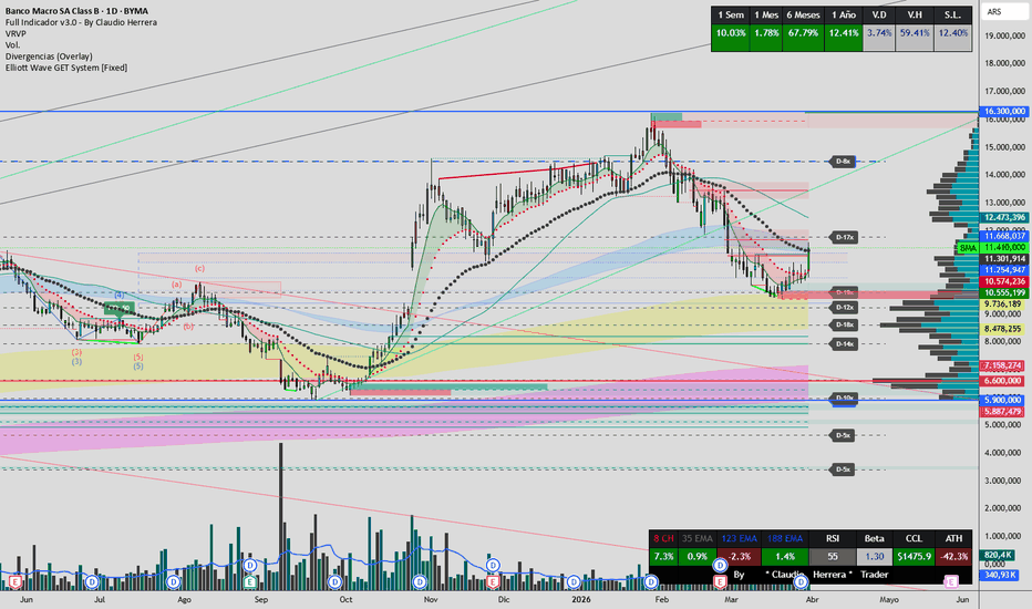
Full Indicador v3.0 - By Claudio HerreraThis script combines several custom indicators to create a configuration that adapts to all timeframes.
The Domenec Tunnel, with its custom, modified moving averages, allows us to always know where we stand. The moving averages and correction tapes, calibrated to fit any chart, provide a visual advantage during analysis, enabling us to quickly recognize trends and critical areas.
The color-coded indicator adds extra value by highlighting "strength/weakness/doubt" in the movement or direction, as well as indicating whether an impulse is strong enough to sustain over time. It allows us to quickly recognize trend exhaustion and reversals.
The inclusion of ICT indicators, support and resistance levels, trend lines, market structure, and FVG detection allows us to identify areas of interest with high volume where the price consistently returns. インジケーター
EZ Oscilator - Live Divergences**How to Trade with EZ Oscillator**
The **EZ Oscillator** combines momentum waves with live divergence detection to deliver clear, high-probability trading signals. Here’s how to use it effectively:
### 1. Bullish Signals (Long Entries)
- **Bullish Crossover**: Look for the fast wave (wt1) crossing **above** the slow signal wave (wt2) when the signal is below 30. This is a strong momentum reversal signal in oversold territory.
- **Bullish Divergence**: A "Bull" label appears when price makes a lower low but the oscillator makes a higher low. This often signals weakening bearish momentum and potential reversal upward.
- Best used near the **Oversold level (15)** or when the oscillator is rising from below the midline (50).
### 2. Bearish Signals (Short Entries)
- **Bearish Crossover**: Look for the fast wave crossing **below** the slow signal wave when the signal is above 70. This indicates momentum exhaustion in overbought territory.
- **Bearish Divergence**: A "Bear" label appears when price makes a higher high but the oscillator makes a lower high. This warns of weakening bullish momentum and possible downward reversal.
- Most effective near the **Overbought level (85)** or when the oscillator is falling from above the midline.
### 3. Key Levels & Confirmation
- **Midline (50)**: Acts as the equilibrium level. Crosses above 50 favor bulls, crosses below 50 favor bears.
- **Overbought (85) / Oversold (15)**: Use dashed levels as dynamic zones. Price + oscillator extremes here increase reversal probability.
- **Divergence Lines**: Visible connecting lines confirm hidden strength or weakness between price and momentum.
### 4. Additional Tips
- The **gradient glow** strengthens visually as the oscillator moves further from 50 — the brighter the glow, the stronger the momentum.
- Combine with higher timeframe context or support/resistance for better accuracy.
- Use the **Trend Bar** at the bottom (if enabled) as a quick visual reference for current momentum direction.
**Pro Tip**: The strongest setups occur when a **crossover** and a **divergence label** appear together near the extreme levels (15 or 85).
This oscillator is non-repainting on closed bars and works across all markets — Forex, Stocks, Crypto, and Futures.
How to Trade with EZ Oscillator
The EZ Oscillator combines momentum waves with live divergence detection to deliver clear, high-probability trading signals. Here’s how to use it effectively:
1. Bullish Signals (Long Entries)
Bullish Crossover : Fast wave (wt1) crosses above the slow signal wave (wt2) when the signal is below 30. Strong momentum reversal in oversold territory.
Bullish Divergence : "Bull" label appears when price makes a lower low but the oscillator makes a higher low — signals weakening bearish momentum.
2. Bearish Signals (Short Entries)
Bearish Crossover : Fast wave crosses below the slow signal wave when the signal is above 70. Indicates momentum exhaustion in overbought territory.
Bearish Divergence : "Bear" label appears when price makes a higher high but the oscillator makes a lower high.
3. Key Levels & Confirmation
Midline (50) : Equilibrium level. Above = bullish bias, Below = bearish bias.
Overbought (85) / Oversold (15) : Use as dynamic reversal zones.
Divergence Lines : Connect pivots to visually confirm hidden strength/weakness.
4. Additional Tips
The gradient glow becomes stronger as the oscillator moves away from 50 — brighter glow = stronger momentum.
Strongest setups occur when a crossover and divergence label appear together near 15 or 85.
Works on all timeframes and markets (Forex, Stocks, Crypto, Futures).
Pro Tip : Always combine with higher timeframe structure or key support/resistance levels for higher probability trades.
The oscillator is non-repainting on closed bars.
インジケーター

[ A L P H A X ] Elliott Wave Detection & Fibonacci Golden ZoneAlphaX Wave – Elliott Wave Detection, Fibonacci Golden Zone Mapping, Multi-Confluence Scoring & Smart SL/TP System
AlphaX Wave is a professional-grade Elliott Wave analysis and trade signal system built on a proprietary multi-engine architecture that fuses automated wave counting, Fibonacci golden zone projection, multi-factor momentum scoring, and structure-based stop loss and target placement into a single cohesive tool. It identifies impulse wave patterns (waves 1–5), detects corrective ABC structures, projects Fibonacci retracement zones, scores trade setups across eight independent confluence factors, and generates graded entry signals with intelligent SL/TP levels derived from swing structure, Fibonacci levels, and wave projections. Designed for traders who use Elliott Wave theory as their primary framework on instruments like XAUUSD, indices, forex majors, and crypto.
━━━━━━━━━━━━━━━━━━━━━━━━━━━━━━━━━━━━━━━━
🔬 The Wave Engine — How It Works
At the core of AlphaX Wave is an automated Elliott Wave detection algorithm that identifies the classical 5-wave impulse structure and 3-wave corrective patterns in real-time. Unlike manual wave counting, this engine applies strict mathematical validation rules derived from Elliott Wave theory to ensure only structurally valid patterns are labeled.
Impulse Wave Detection (Waves 1–5)
The engine uses a rolling buffer of confirmed swing highs and swing lows detected via a configurable pivot lookback. When at least three swing highs and three swing lows are available, the engine tests them against the following Elliott Wave rules:
Wave 2 must not retrace beyond the start of Wave 1 — validated by checking that the second swing low remains above the first swing low (bullish) or below the first swing high (bearish)
Wave 3 must not be the shortest impulse wave — validated by comparing the Wave 3 range to at least 70% of the Wave 1 range
Wave 4 must not overlap into Wave 1 territory — validated by checking that the Wave 4 low stays above the Wave 2 low (bullish) or Wave 4 high stays below the Wave 2 high (bearish)
Wave 2 retracement must be between 15% and 95% of Wave 1 — filters out patterns that are too shallow or too deep
Wave 4 retracement must be between 10% and 90% of Wave 3 — ensures proper proportionality
Temporal ordering must be correct — all six pivot points must occur in strict chronological sequence
Wave 5 must exceed Wave 3's high (bullish) or undercut Wave 3's low (bearish) — confirms the impulse completed with a new extreme
When all rules pass simultaneously, the engine marks the complete 1–5 impulse structure on the chart with numbered labels and connecting wave lines. Wave 3 and Wave 5 receive larger, brighter labels because they represent the highest-momentum phases of the impulse.
Corrective Wave Detection (ABC Pattern)
After an impulse completes, the engine monitors for corrective price action:
For a completed bullish impulse — the engine watches for a pullback that retraces between 20% and 72% of the impulse range, indicating an ABC correction is forming
For a completed bearish impulse — the engine watches for a bounce that retraces between 20% and 72% of the impulse range
The correction must originate after Wave 5 completes — ensures proper sequence
A configurable cooldown prevents multiple correction labels from firing on the same structure
Corrective zones are particularly valuable because they represent potential entry opportunities in the direction of the prior impulse trend — the market is pulling back within a larger trend structure.
━━━━━━━━━━━━━━━━━━━━━━━━━━━━━━━━━━━━━━━━
📐 Fibonacci Golden Zone System
When an impulse wave completes, the engine automatically projects Fibonacci retracement levels across the entire impulse range:
38.2% Retracement — the shallowest institutional retracement level
50.0% Retracement — the equilibrium midpoint of the impulse
61.8% Retracement — the golden ratio level, highest-probability reversal zone
The area between the 38.2% and 61.8% levels forms the Golden Zone — a shaded box that represents the highest-probability area for the corrective wave to terminate and the trend to resume. This is where institutional traders typically place their limit orders.
The Golden Zone system includes intelligent lifecycle management:
Zones automatically expire after a configurable maximum age (default 80 bars)
Zones are removed when price closes significantly beyond them (1.5 ATR past the zone boundary) — indicating the zone has been invalidated
Maximum active zones are capped (configurable) to keep the chart clean
The indicator tracks whether price is currently inside a bullish or bearish Golden Zone — this information feeds directly into the confluence scoring engine
━━━━━━━━━━━━━━━━━━━━━━━━━━━━━━━━━━━━━━━━
📊 Wave 3 Setup Detection
Wave 3 is traditionally the strongest and longest wave in Elliott Wave theory. AlphaX Wave includes a dedicated Wave 3 Setup Scanner that identifies potential Wave 3 initiations in real-time:
Detects when price has completed a valid Wave 1 (impulse move) followed by a Wave 2 (pullback between 15% and 90% of Wave 1)
Confirms the pullback low remains above the Wave 1 starting point (bullish) or below it (bearish) — validating the wave structure
Requires a directional confirmation candle (close above prior high for bullish, close below prior low for bearish)
Marked with small purple triangles — ▲ below bar for bullish Wave 3 setups, ▼ above bar for bearish
Wave 3 setups are among the highest-probability trade entries in all of technical analysis because they align with the strongest phase of the impulse trend.
━━━━━━━━━━━━━━━━━━━━━━━━━━━━━━━━━━━━━━━━
🧠 8-Factor Confluence Scoring Engine
Every potential trade signal is evaluated across eight independent confluence factors . Each factor scores either 0 or 1 point, producing a confluence score from 0 to 8. Only signals meeting your configured minimum confluence threshold are displayed.
Factor 1 — Wave 3 Setup (W3)
Is a valid Wave 3 initiation pattern present?
This is the single most powerful factor — Wave 3 moves are the strongest in Elliott theory
Factor 2 — ABC Correction Zone (ABC)
Is the market currently in a corrective phase following a completed impulse?
Corrections within trends offer the best risk/reward entries
Factor 3 — Price in Fibonacci Golden Zone (FIB)
Is price currently inside an active Golden Zone box (between 38.2% and 61.8% retracement)?
Golden Zone entries have institutional backing
Factor 4 — Price at Specific Fibonacci Level (FLV)
Is price at or near the 38.2%, 50.0%, or 61.8% retracement level specifically?
Precision Fibonacci entries add edge beyond just being "in the zone"
Factor 5 — Momentum Alignment (MOM)
Are RSI slope, MACD direction, MACD histogram momentum, and Stochastic all aligned in the signal direction?
Requires at least 2 of 5 momentum sub-factors to confirm
Factor 6 — RSI Divergence (DIV)
Is a confirmed RSI divergence present (price makes new low but RSI makes higher low, or vice versa)?
Divergence is one of the most reliable reversal confirmation signals
Factor 7 — Volume Confirmation (VOL)
Is current volume above the moving average with a candle closing in the signal direction?
Volume validates institutional participation in the move
Factor 8 — EMA Trend Alignment (EMA)
Are the Fast (21), Medium (50), and Slow (200) EMAs properly stacked in the signal direction?
Or is price at least above/below the 200 EMA with Fast above/below Medium?
━━━━━━━━━━━━━━━━━━━━━━━━━━━━━━━━━━━━━━━━
📊 Confidence Scoring & Grade System
Beyond the 8-factor confluence count, each signal receives a weighted confidence score from 0 to 100% that reflects the quality and strength of the setup:
Wave Structure (up to 22 points)
Wave 3 Setup present = 22 points (highest single contributor)
ABC Correction active = 12 points
Fibonacci Alignment (up to 22 points)
Price inside Golden Zone = 15 points
Price at 61.8% level = 7 points, at 50.0% = 5 points, at 38.2% = 4 points
Momentum Confirmation (up to 23 points)
Momentum aligned (2+ sub-factors) = 12 points
Strong momentum (4+ sub-factors) = additional 6 points
MACD crossover on signal bar = 5 points
RSI Analysis (up to 14 points)
RSI divergence confirmed = 10 points
RSI slope in ideal range = 4 points
RSI already at opposite extreme (penalty) = -5 points
Volume & Trend (up to 20 points)
Volume above average + directional candle = 5 points
Volume spike + directional candle = 3 points
Full EMA alignment (Fast > Medium > Slow or reverse) = 8 points
Cloud direction confirmed = 4 points
Signals are classified into grades based on the final confidence score:
A+ Grade (70%+) — Exceptional setup. Maximum confluence across wave structure, Fibonacci, momentum, and trend.
A Grade (55–69%) — High-quality setup. Most major factors aligned.
B Grade (40–54%) — Solid setup. Core conditions met with moderate confirmation.
C Grade (25–39%) — Marginal setup. Basic conditions met but weaker confirmation. Hidden by default.
D Grade (below 25%) — Weak setup. Minimal confluence. Hidden by default.
━━━━━━━━━━━━━━━━━━━━━━━━━━━━━━━━━━━━━━━━
📊 Signal Labels — What They Show
Each entry signal label displays comprehensive information in a compact format:
Direction — ▲ LONG or ▼ SHORT with spaced lettering
Grade — A+, A, B, C, or D classification
Confidence Percentage — The weighted score from the confidence engine
Confluence Count — How many of the 8 factors are active (e.g., 5/8)
Active Factor Checklist — Shows exactly which factors contributed: ✓W3 ✓ABC ✓FIB ✓FLV ✓MOM ✓DIV ✓VOL ✓EMA
Label colors follow the grade system:
Bull signals — Bright green (A+), Primary green (A), Dim green (B), Neutral gray (C/D). All use dark text for readability.
Bear signals — Bright red (A+), Primary red (A), Dim red (B), Neutral gray (C/D). All use white text for readability.
A thin dotted line connects the signal label to the price bar, keeping the label offset from price action to avoid chart clutter.
━━━━━━━━━━━━━━━━━━━━━━━━━━━━━━━━━━━━━━━━
🎯 Smart SL/TP System — Structure-Based Risk Management
Every entry signal automatically generates three trade management levels — Stop Loss, Target 1, and Target 2 — using a multi-source calculation engine that prioritizes structural price levels over arbitrary ATR multiples.
Stop Loss Calculation
The SL engine searches for the optimal stop placement using this priority cascade:
Nearest swing structure — Finds the closest confirmed swing low (for longs) or swing high (for shorts) within a 50-bar lookback. Places the SL beyond this level with ATR padding.
ATR floor and cap — Ensures the SL is never too tight (70% of base ATR multiple) or too wide (180% of base ATR multiple) regardless of swing structure.
Confidence modifier — Higher-grade signals receive tighter stops (0.85× for A+, 0.92× for A, 1.0× for B, 1.15× for C/D). This reflects the higher-probability nature of strong setups.
Target 1 Calculation
TP1 represents the conservative take-profit level:
Nearest opposing swing — Searches for the closest swing high above entry (longs) or swing low below entry (shorts) that provides at least 1.2× the SL distance.
Fibonacci level targeting — If an active Fibonacci zone has a 38.2% or 50.0% level above/below entry that provides better targeting than the swing level, the Fib level is used.
Minimum R:R enforcement — TP1 is guaranteed to provide at least the configured ATR multiple (default 2.5×) of risk-reward.
Target 2 Calculation
TP2 represents the extended profit target:
Wave-based projection — If an impulse wave is active, TP2 is calculated as 61.8% of the total impulse range — representing the typical next-wave target.
Far swing structure — Searches for swing levels further than TP1 that provide at least 1.3× the TP1 distance.
Fibonacci extension — If the 61.8% Fibonacci level provides a target beyond TP1, it is used as TP2.
Minimum spacing — TP2 is guaranteed to be at least 1.5× the TP1 distance from entry.
Break-Even Protection
When TP1 is hit, the system automatically adjusts the Stop Loss to the entry price (break-even). The SL label changes to "BE" with a neutral color, visually confirming that the trade is now risk-free on the remaining position targeting TP2.
Hit Tracking
All SL/TP levels are tracked in real-time:
When a level is hit, the label changes color — red fill for SL hits, green fill for TP hits
SL hits are processed first — if the SL is hit, TP levels for that trade are no longer tracked
TP1 must be hit before TP2 tracking activates the break-even mechanism
Historical SL/TP groups are automatically trimmed to keep the chart clean (configurable history count)
━━━━━━━━━━━━━━━━━━━━━━━━━━━━━━━━━━━━━━━━
📐 Trend Context Layer
Three independent trend analysis systems provide structural context:
Triple EMA System
Fast EMA (21) — Yellow-green crosses. Immediate momentum reference.
Medium EMA (50) — Gray line. Intermediate trend filter.
Slow EMA (200) — Dark gray, thicker line. Macro structural backbone used in confidence scoring.
When all three are properly stacked (Fast > Medium > Slow for bullish, reverse for bearish), trend alignment scores maximum points.
Trend Cloud
Calculated from the midpoints of the highest high / lowest low over fast (9) and slow (26) periods
When the fast midpoint is above the slow midpoint, the cloud fills green — bullish bias
When below, the cloud fills red — bearish bias
Cloud direction adds 4 points to the confidence score when aligned with the signal
RSI Divergence System
Detects classical RSI divergence using pivot-based comparison
Bullish divergence — price makes a lower low but RSI makes a higher low
Bearish divergence — price makes a higher high but RSI makes a lower high
Divergence must occur within a valid lookback window (5–50 bars between pivots) and be recent (within 3 bars of the current RSI pivot)
Marked with small diamond shapes — green below bar for bullish, red above bar for bearish
━━━━━━━━━━━━━━━━━━━━━━━━━━━━━━━━━━━━━━━━
📊 Momentum Engine
The momentum engine combines four oscillator systems into a unified momentum score:
RSI Slope — Smoothed RSI direction over 2 bars. Bullish when RSI is between 40–75 and rising. Bearish when RSI is between 25–60 and falling.
MACD Direction — MACD Line above Signal Line = bullish, below = bearish.
MACD Histogram Momentum — Histogram increasing = bullish momentum, decreasing = bearish momentum.
Stochastic Alignment — %K above %D with room to run (below 80) = bullish. %K below %D with room to fall (above 20) = bearish.
MACD Crossover — Fresh MACD crossover on the signal bar adds additional confirmation.
Scores of 2+ out of 5 confirm momentum alignment. Scores of 4+ indicate strong momentum — adding bonus points to the confidence score.
━━━━━━━━━━━━━━━━━━━━━━━━━━━━━━━━━━━━━━━━
📐 Dashboard Intelligence
A comprehensive 3-column AlphaX-branded dashboard provides real-time analysis across all engine layers:
Wave & Fibonacci Status
Current wave phase — Impulse 1–5 (detected/active), Corrective ABC, or Scanning
Wave trend direction — Bullish or Bearish impulse context
Fibonacci status — In Golden Zone, at specific level, or no active zone
Active Fibonacci zone count
Momentum & Trend
Momentum state — Strong Bull/Bear, Bullish/Bearish, or Flat
Bull/Bear sub-factor scores (e.g., 3▲ 1▼)
EMA trend alignment — Bull Aligned, Bear Aligned, or Mixed
Price position relative to 200 EMA
Cloud direction — Bullish, Bearish, or Flat
Volume & Oscillators
Relative volume — Spike, High, Normal, or Dry with exact ratio
RSI state — Overbought, Oversold, Rising, Falling, or Neutral with numeric value
Confluence & Verdict
Bull confluence score — count out of 8, confidence percentage, and letter grade
Bear confluence score — count out of 8, confidence percentage, and letter grade
Verdict — the engine's overall assessment: High Confidence Long, High Confidence Short, Lean Long/Short with Caution, Mixed — Stand Aside, or No Clear Edge
━━━━━━━━━━━━━━━━━━━━━━━━━━━━━━━━━━━━━━━━
🚀 How to Trade with AlphaX Wave — Step by Step
Step 1 — Identify the Wave Structure
Look for completed impulse patterns (numbered 0–5 on the chart)
Check the Dashboard: What is the current Wave Phase?
If "SCANNING" — no valid wave structure detected yet. Wait for pattern formation.
Step 2 — Wait for Correction or Wave 3 Setup
After an impulse completes, watch for the "ABC CORRECTION ZONE" label — this is where the market is pulling back within the trend
Watch for Wave 3 Setup triangles (▲/▼) — these mark the beginning of the strongest wave
Check if price is entering a Fibonacci Golden Zone (purple shaded box)
Step 3 — Enter on Confluence Signal
Wait for a graded entry label (▲ LONG or ▼ SHORT) to appear
Check the grade — A+ and A signals have the highest probability
Review the factor checklist — more ✓ marks = stronger setup
The SL and TP levels are automatically plotted for immediate trade management
Step 4 — Manage the Trade
Monitor the SL/TP levels on the chart — they update automatically
When TP1 is hit, the label lights up green and the SL moves to break-even
Hold the remaining position for TP2 risk-free
If SL is hit first, the label turns red — accept the loss and wait for the next setup
Step 5 — Read the Verdict
The Dashboard Verdict row summarizes the engine's real-time assessment
"HIGH CONFIDENCE LONG/SHORT" — all systems aligned, actively look for entries
"LEAN LONG/SHORT — CAUTION" — some alignment but not full, trade with reduced size
"MIXED — STAND ASIDE" — conflicting signals, do not trade
"NO CLEAR EDGE" — insufficient data, wait for structure to develop
━━━━━━━━━━━━━━━━━━━━━━━━━━━━━━━━━━━━━━━━
⚠ When NOT to Trade — Reading the Warning Signs
Dashboard shows "SCANNING" — No valid wave structure detected. The market may be in a complex correction or transition phase.
Verdict shows "MIXED — STAND ASIDE" — Bull and bear confluence are both active simultaneously. Conflicting signals cancel each other.
Cloud is flat or rapidly switching colors — No established trend direction. Signals during cloud transitions are less reliable.
EMAs are tangled and flat — Range-bound market. Wave patterns in choppy conditions produce lower-quality signals.
Only C or D grade signals appearing — Insufficient confluence. These grades are hidden by default for a reason.
RSI showing "OVERBOUGHT" on a long signal — The confidence engine already penalizes this (-5 points), but it is worth noting visually as well.
Volume showing "DRY" — Low-volume environments reduce the reliability of all technical patterns including waves.
━━━━━━━━━━━━━━━━━━━━━━━━━━━━━━━━━━━━━━━━
⚡ Key Features
🔬 Automated Elliott Wave impulse detection (1–5) with strict rule validation
📐 ABC corrective pattern recognition with retracement depth validation
🎯 Wave 3 Setup Scanner — identifies the strongest wave initiation points
📊 Fibonacci Golden Zone projection with intelligent lifecycle management
🧠 8-factor confluence scoring — Wave, ABC, Fibonacci, Fibonacci Level, Momentum, Divergence, Volume, EMA
📈 Weighted confidence scoring (0–100%) with A+ through D grade classification
▲▼ Detailed signal labels showing grade, confidence, confluence count, and active factor checklist
🎯 Structure-based SL/TP system — swing levels, Fibonacci targets, and wave projections
🛡 Automatic break-even protection when TP1 is hit
📊 Real-time hit tracking with visual color changes on SL/TP labels
☁ Trend Cloud with gradient fill for instant directional bias
📐 Triple EMA system (21/50/200) for structural trend context
💎 RSI divergence detection with pivot-based validation
📊 Multi-oscillator momentum engine (RSI, MACD, Stochastic)
📊 Volume spike detection with configurable multiplier
📐 Comprehensive 3-column dashboard with verdict system
🎨 Cohesive triple-tone color theme — Green for bull, Red for bear, Purple for wave structure
🔔 10 alert conditions — signals, impulses, corrections, Wave 3 setups, and divergences
⚙ Fully configurable — wave detection, Fibonacci, momentum, signals, SL/TP, and all visuals
━━━━━━━━━━━━━━━━━━━━━━━━━━━━━━━━━━━━━━━━
⚙ Settings Reference
Wave Detection
Swing Detection Length — Pivot lookback for identifying swing highs and lows (default: 6)
Show Wave Count Labels — Toggle the numbered 0–5 labels on impulse waves
Show Wave Structure Lines — Toggle the connecting lines between wave points
Show Impulse Completion — Toggle the "IMPULSE COMPLETE" notification labels
Show Corrective Patterns — Toggle the "ABC CORRECTION ZONE" labels
Show Wave 3 Setup Markers — Toggle the purple triangle markers
Wave Pattern Cooldown — Minimum bars between wave pattern detections (default: 18)
Fibonacci
Show Fib Golden Zone Boxes — Toggle the shaded 38.2%–61.8% retracement zone
Max Fib Zone Boxes — Maximum simultaneous Golden Zones (default: 3)
Fib Zone Max Age — Bars before a zone auto-expires (default: 80)
Momentum
RSI Length / Smoothing — Core RSI calculation parameters
MACD Fast / Slow / Signal — MACD oscillator parameters
Show RSI Divergence — Toggle divergence diamond markers
Volume
Volume MA Length — Baseline period for volume comparison (default: 20)
Volume Spike Multiplier — Threshold for spike detection (default: 1.6×)
Show Volume Spike Dots — Toggle volume spike indicators at bar bottom
EMA Settings
Fast / Medium / Slow EMA — Independently toggle visibility and set periods
Defaults: 21 / 50 / 200
Trend Cloud
Show Trend Cloud — Toggle the gradient cloud fill
Cloud Fast / Slow Length — Midpoint calculation periods (default: 9 / 26)
Confluence Engine
Min Confluence Score — Minimum factors required for a signal (default: 3 of 8)
Show Entry Signals — Toggle signal labels
Signal Cooldown — Minimum bars between signals (default: 10)
Signal Label Offset — Distance below/above bar in ATR units (default: 3.0)
Show Grade C / D Signals — Toggle lower-quality signal visibility (default: off)
SL / TP
Show Stop Loss & Targets — Toggle all SL/TP visual elements
Stop Loss (× ATR) — Base ATR multiple for stop loss calculation (default: 2.0)
Target 1 (× ATR) — Base ATR multiple for conservative target (default: 2.5)
Target 2 (× ATR) — Base ATR multiple for extended target (default: 5.0)
Limit SL/TP History — Cap the number of visible historical trade levels
SL/TP History Count — Maximum trade groups shown (default: 8)
Move SL to Break Even after TP1 — Enable/disable break-even protection
Display
Show Dashboard — Toggle the information panel
Dashboard Position — Top Right, Top Left, Bottom Right, Bottom Left
Dashboard Text Size — Tiny, Small, Normal
Dashboard Background — Background color for the panel
Theme Colors
Bull Primary / Bright / Dim — Green family for bullish elements
Bear Primary / Bright / Dim — Red family for bearish elements
Wave Primary / Bright / Dim — Purple family for wave structure elements
Fibonacci Levels / Dim — Purple-pink family for Fibonacci zones
EMA colors — Fast (green), Medium (gray), Slow (dark gray)
Neutral — Gray for inactive/mixed states
━━━━━━━━━━━━━━━━━━━━━━━━━━━━━━━━━━━━━━━━
🔔 Alert Conditions
Wave Long Signal — Fires when a graded bullish entry signal appears
Wave Short Signal — Fires when a graded bearish entry signal appears
Bullish Impulse Complete — Fires when a full 1–5 bullish impulse is detected
Bearish Impulse Complete — Fires when a full 1–5 bearish impulse is detected
Wave 3 Bull Setup — Fires when a bullish Wave 3 initiation pattern is detected
Wave 3 Bear Setup — Fires when a bearish Wave 3 initiation pattern is detected
RSI Bull Divergence — Fires when bullish RSI divergence is confirmed
RSI Bear Divergence — Fires when bearish RSI divergence is confirmed
Bullish ABC Correction — Fires when a bullish corrective zone is identified
Bearish ABC Correction — Fires when a bearish corrective zone is identified
All alert messages include {{ticker}} and {{interval}} placeholders for clean webhook integration.
━━━━━━━━━━━━━━━━━━━━━━━━━━━━━━━━━━━━━━━━
🎯 Default Settings — Optimized For
The default configuration is tuned for XAUUSD (Gold) and major instruments on the 5-minute to 1-hour timeframes :
Swing Length at 6 captures wave structure without excessive lag on intraday charts
Minimum confluence at 3/8 ensures signals have meaningful multi-factor backing
Signal cooldown at 10 bars prevents rapid-fire signals during volatile wave transitions
SL at 2.0 ATR with structure-based adjustment provides adaptive risk sizing
TP1 at 2.5 ATR and TP2 at 5.0 ATR provide minimum 1.25R and 2.5R risk-reward ratios
Break-even protection ensures profitable trades are protected after TP1
Grade C and D signals hidden by default to maintain signal quality
For other instruments or timeframes, adjust:
Higher timeframes (4H, Daily) — Increase Swing Length to 8–14, increase Wave Cooldown to 30–50, increase SL/TP ATR multiples
Lower timeframes (1m) — Reduce Swing Length to 4–5, reduce Signal Cooldown to 5–7, increase Min Confluence to 4
Forex majors — Use defaults, optionally reduce Swing Length to 5 for tighter wave detection
Crypto — Increase Swing Length to 8–10 (higher volatility), increase SL ATR multiple to 2.5–3.0
Fewer, higher-quality signals — Increase Min Confluence to 4–5, increase Signal Cooldown, hide Grade C/D
More signals — Reduce Min Confluence to 2, enable Grade C signals, reduce cooldown
━━━━━━━━━━━━━━━━━━━━━━━━━━━━━━━━━━━━━━━━
👥 Who This Is For
📐 Elliott Wave Practitioners — Automated wave counting with strict rule validation eliminates subjective bias
📊 Fibonacci Traders — Automatic Golden Zone projection with lifecycle management removes manual drawing
🥇 Gold & Forex Intraday Traders — Optimized for instruments with clean wave structures on fast timeframes
🧠 Systematic Traders — The 8-factor confluence + weighted confidence system provides a fully quantitative framework
🎯 Traders who want complete trade plans — Entry, SL, TP1, TP2, and break-even all generated automatically
📈 Traders learning Elliott Wave — The visual wave labels and structure lines serve as an educational overlay
⚠ Traders who struggle with exit management — The SL/TP system with hit tracking and break-even automation removes emotional decision-making
━━━━━━━━━━━━━━━━━━━━━━━━━━━━━━━━━━━━━━━━
📝 Notes
Wave detection uses confirmed pivot points (offset by the swing length) — wave labels appear after structural confirmation, not in real-time. This prevents repainting.
The indicator requires sufficient bar history to populate swing buffers — allow at least 100+ bars of data before expecting wave pattern detection
Elliott Wave rules are applied as mathematical approximations of the classical theory — certain complex wave structures (extended waves, truncations, diagonal triangles) may not be detected
SL/TP levels are calculated at signal time and do not adjust afterward (except the break-even mechanism on TP1 hit)
Maximum 500 labels, 500 lines, and 500 boxes are used — on very low timeframes with extended history and many signals, oldest drawings may be automatically removed by TradingView's rendering limits
The SL/TP history is automatically trimmed to the configured limit (default 8 trade groups = 24 labels/lines) to stay within TradingView's drawing limits
All confluence factors and confidence scores are recalculated on every bar — the dashboard reflects the current bar's state, not the last signal's state
━━━━━━━━━━━━━━━━━━━━━━━━━━━━━━━━━━━━━━━━
⚠ Disclaimer
This indicator is a technical analysis and visualization tool intended for educational and informational purposes only. It does not constitute financial advice or a recommendation to buy or sell any financial instrument. Elliott Wave patterns, Fibonacci levels, and all signals are generated from historical and real-time price data using mathematical calculations — their accuracy or profitability is not guaranteed. Elliott Wave theory is inherently subjective and interpretive; automated detection provides one possible wave count among many valid alternatives. Past wave patterns and signal performance do not guarantee future results. Always conduct your own analysis, use proper risk management, and consult a licensed financial advisor before making any trading decisions. The author accepts no responsibility for any losses incurred from the use of this indicator.
━━━━━━━━━━━━━━━━━━━━━━━━━━━━━━━━━━━━━━━━
Built for traders who demand clarity, confidence, and precision from their charts. インジケーター

Displacement Lens [JOAT]Displacement Lens
Introduction
The Displacement Lens is an advanced open-source momentum analysis indicator that measures real-time displacement intensity by fusing four normalized momentum oscillators with volume-weighted candle body analysis. It produces a composite displacement score displayed as a gradient histogram with adaptive threshold bands, designed to separate institutional displacement candles from retail noise. This is not a simple oscillator mashup — it is a unified displacement measurement engine with institutional-grade features built on top of the core signal.
The indicator operates in its own pane (non-overlay) and provides traders with a clear, visual representation of when price is being displaced by institutional force versus when it is drifting on low-conviction retail flow.
Why This Indicator Exists
Standard momentum oscillators like RSI, CCI, or Bollinger %B each capture only one dimension of market momentum. Traders often flip between multiple oscillators trying to get a complete picture. The Displacement Lens solves this by:
Normalizing four independent oscillators (BB %B, CCI, ROC, RSI) to a common scale so they can be meaningfully combined
Weighting the composite by volume intensity and candle body ratio — because a large-bodied candle on high volume is institutional displacement, while a small-bodied candle on low volume is noise
Adding adaptive threshold bands that adjust to the signal's own volatility, rather than using fixed overbought/oversold levels that fail in different market conditions
Layering institutional features on top: decay detection, accumulation phases, divergence scanning, exhaustion markers, and a per-bar institutional candle grade
The result is a single composite signal that tells you not just "is momentum bullish or bearish" but "how strong is the institutional displacement right now, and is it accelerating, decaying, or exhausting?"
Core Signal Construction
The displacement signal is built in three stages:
Stage 1: Oscillator Normalization
Each of the four oscillators is normalized to a range using methods appropriate to each:
Bollinger %B: Measures where price sits within the Bollinger Bands. The raw %B (0 to 1) is remapped to with a soft clamp. When price is above the upper band, the score approaches +1. Below the lower band, it approaches -1.
CCI: The Commodity Channel Index is divided by 200 and clamped. CCI values beyond +/-200 saturate at +/-1, while values near zero produce scores near zero.
ROC: Rate of Change is normalized using adaptive scaling — it divides by twice its own standard deviation over 50 bars. This means the normalization adapts to the instrument's typical momentum range.
RSI: Remapped from the standard 0-100 range to by subtracting 50 and dividing by 50. RSI 70 becomes +0.4, RSI 30 becomes -0.4.
Each oscillator can be individually toggled on or off, and the composite averages only the active ones.
Stage 2: Volume-Weighted Displacement
The oscillator composite is blended with a volume displacement component:
float vol_displacement = disp_direction * body_ratio * vol_intensity
float raw_signal = osc_composite * (1.0 - vol_weight) + vol_displacement * vol_weight
Where:
disp_direction is +1 for bullish candles, -1 for bearish
body_ratio is the candle body size divided by the full range (high-low) — institutional candles have ratios above 0.7
vol_intensity is current volume relative to the 20-bar average, clamped to
vol_weight (default 0.3) controls how much volume influences the final score
This means a strong oscillator reading on a small-bodied, low-volume candle gets dampened, while a moderate oscillator reading on a large-bodied, high-volume candle gets amplified.
Stage 3: Smoothing and Thresholds
The raw signal is smoothed with an EMA (default period 5), and adaptive threshold bands are calculated as the signal's own standard deviation multiplied by a configurable factor (default 1.5x over 100 bars). This creates bands that widen in volatile markets and tighten in calm markets — far more reliable than fixed thresholds.
Institutional Features
1. Displacement Impulse Signals
When the signal crosses above the upper threshold for the first time (with volume and body confirmation), a bullish impulse label appears. Similarly for bearish. These mark the exact moment institutional displacement begins — not after it has already played out.
2. Momentum Divergence Engine
The indicator detects four types of divergence between price pivots and signal pivots:
Regular Bearish: Price makes a higher high, but the displacement signal makes a lower high — momentum is weakening despite price advance
Regular Bullish: Price makes a lower low, but the signal makes a higher low — selling pressure is fading
Hidden Bearish: Price makes a lower high, but the signal makes a higher high — continuation of downtrend likely
Hidden Bullish: Price makes a higher low, but the signal makes a lower low — continuation of uptrend likely
Divergences are detected using configurable pivot lengths and drawn as labeled markers directly on the histogram.
3. Displacement Decay Zones
When the signal was above the upper threshold but starts declining (still positive, but fading), the indicator marks a "decay zone" — a dotted box on the histogram showing where institutional momentum is waning. This is a unique concept: it identifies the transition from impulse to drift before the signal crosses zero. Bear decay zones work identically on the downside.
4. Accumulation Phase Detector
When both the signal and signal line are near zero (below half the standard deviation) for a minimum number of bars, the indicator draws a dashed "accumulation" box. These low-displacement consolidation phases often precede the next major impulse move. The concept is borrowed from Wyckoff methodology but applied to displacement scoring rather than price.
5. Institutional Candle Grading
Every bar receives a grade from D to A+ based on three factors:
Body ratio (how much of the candle is body vs wick) — 33.3% weight
Volume intensity (current volume vs 20-bar average) — 33.3% weight
Displacement alignment (how far the signal is from the threshold) — 33.4% weight
A+ candles (score >= 80) with body ratio > 0.7 and volume > 1.5x average are flagged as true institutional candles. The grade is shown in the dashboard.
6. Velocity Channel
The rate of change of the displacement signal itself is plotted as a velocity line with standard deviation bands. When velocity is expanding (accelerating), the displacement move has conviction. When velocity contracts, the move is losing steam. Optional glow effects make the velocity channel visually distinct.
7. Exhaustion Detection
Bullish exhaustion fires when the signal was above the threshold for 3 consecutive bars and then declines for 3 consecutive bars. Bearish exhaustion is the mirror. These are rare, high-conviction reversal signals that mark the exact point where institutional displacement has peaked and is reversing.
8. HTF Displacement Bias
The indicator calculates the same displacement composite on a higher timeframe (default 4H) using request.security(). When the current timeframe signal aligns with the HTF bias, conviction is higher. The dashboard shows whether HTF is BULLISH, BEARISH, or NEUTRAL and whether it is aligned with the current signal.
9. Displacement Streak Counter
Tracks how many consecutive bars the signal has been above the upper threshold (bull streak) or below the lower threshold (bear streak). Longer streaks indicate sustained institutional pressure.
Visual Elements
Gradient Histogram: The main displacement signal plotted as columns with gradient coloring — bullish bars transition from muted teal to bright teal as strength increases, bearish bars from muted rose to hot rose. Volume spike bars are highlighted in amber.
Signal Line: A further-smoothed version of the signal (3x the smoothing period) plotted as a bright lavender line. Crossovers between the signal and signal line generate diamond markers.
Adaptive Threshold Bands: Upper and lower threshold lines that expand and contract with signal volatility.
Decay Zones: Dotted boxes marking fading institutional momentum.
Accumulation Zones: Dashed boxes marking low-displacement consolidation.
Velocity Channel: Rate-of-change line with glow bands showing displacement acceleration.
15-Row Dashboard: Comprehensive command center showing Signal value, Phase classification, Candle Grade, HTF Bias, Streak, Velocity, Divergence status, and more.
Input Parameters
Oscillator Components:
BB Length (default 20), BB Multiplier (default 2.0)
CCI Length (default 23), ROC Length (default 50), RSI Length (default 14)
Individual toggles for each oscillator
Displacement Engine:
Signal Smoothing (default 5) — EMA period for the final signal
Volume Weight (default 0.3) — how much volume influences the score
Threshold Lookback (default 100) — period for adaptive threshold calculation
Threshold Multiplier (default 1.5) — sensitivity of threshold bands
Institutional Features:
Toggles for Impulse Signals, Divergences, Decay Zones, Accumulation Phases, Signal Crossovers, Velocity Channel, Exhaustion Markers, HTF Bias
HTF Timeframe (default 240 / 4H)
Accumulation Min Bars (default 8), Decay Min Bars (default 5)
Max Boxes (default 30), Divergence Pivot Length (default 5)
How to Use This Indicator
Step 1: Read the Phase
The dashboard shows the current displacement phase: IMPULSE BULL, IMPULSE BEAR, DRIFT BULL, DRIFT BEAR, DECAY, ACCUMULATION, or FLAT. This tells you the market's current displacement state at a glance.
Step 2: Watch for Impulse Signals
When the signal crosses the threshold with volume confirmation, an impulse label appears. These are the highest-conviction displacement events — institutional money is moving price.
Step 3: Monitor Decay and Exhaustion
After an impulse, watch for decay zones forming. If the signal was strong and starts declining, the move is losing institutional backing. Exhaustion markers confirm the reversal point.
Step 4: Confirm with HTF Bias
Check whether the HTF displacement aligns with the current timeframe. Aligned signals have higher follow-through probability.
Step 5: Use Divergences for Reversals
Regular divergences warn of potential reversals. Hidden divergences confirm trend continuation. Both are detected automatically.
Step 6: Identify Accumulation for Breakout Setups
When the indicator marks an accumulation phase (low displacement for extended bars), prepare for the next impulse. The breakout direction is often confirmed by the first impulse signal after accumulation ends.
Limitations
The indicator measures displacement intensity, not price direction prediction. Strong displacement can occur in both breakouts and fakeouts.
Volume data quality varies by instrument and exchange. Forex volume on TradingView represents tick volume, not true volume.
HTF bias uses request.security() which may produce different results on different chart types.
Divergence detection requires sufficient pivot history — it will not fire on the first few hundred bars of a chart.
Exhaustion signals are intentionally rare (require 3 bars above threshold + 3 bars declining). They may not fire in fast-moving markets.
The indicator works best on liquid instruments with consistent volume patterns.
Past displacement patterns do not guarantee future price movement.
Originality Statement
This indicator is original in its unified displacement measurement approach. While individual oscillators (BB %B, CCI, ROC, RSI) are well-known, this indicator is justified because:
It normalizes four oscillators to a common scale using methods appropriate to each (adaptive scaling for ROC, division-based for CCI, remapping for RSI and BB %B) — not simply averaging raw values
The volume-weighted displacement component integrates candle body analysis with volume intensity, creating a measure that distinguishes institutional candles from retail noise
Adaptive threshold bands based on the signal's own standard deviation replace unreliable fixed thresholds
The Displacement Decay Zone concept — identifying the transition from impulse to drift before the signal crosses zero — is not available in standard oscillators
The Accumulation Phase Detector applies Wyckoff-inspired consolidation detection to a composite momentum score rather than price
The Institutional Candle Grading system scores every bar on three dimensions simultaneously (body, volume, displacement alignment)
The Velocity Channel measures the rate of change of displacement itself — a second derivative that reveals acceleration and deceleration of institutional activity
The combination of all these features with a comprehensive dashboard creates a unified displacement analysis system not available in any single existing indicator
Disclaimer
This indicator is provided for educational and informational purposes only. It is not financial advice or a recommendation to buy or sell any financial instrument. Trading involves substantial risk of loss and is not suitable for all investors.
The displacement signal measures momentum intensity based on mathematical calculations of current and historical market data. It does not predict future price movement. High displacement does not guarantee profitable trades. Past displacement patterns do not guarantee future patterns.
Always use proper risk management, including stop losses and position sizing appropriate for your account size and risk tolerance. Never risk more than you can afford to lose.
The author is not responsible for any losses incurred from using this indicator. Users assume full responsibility for all trading decisions.
-Made with passion by officialjackofalltrades
インジケーター

インジケーター
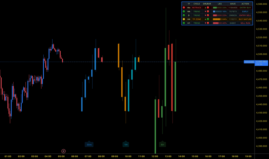
Singularity Convergence Protocol [JOAT]Singularity Convergence Protocol
Introduction
The Singularity Convergence Protocol is an advanced open-source multi-system confluence strategy that combines eight distinct analytical methodologies into a unified trading system. This strategy integrates momentum analysis, Smart Money Concepts, velocity waves, liquidity tracking, trend detection, divergence analysis, volatility measurement, and institutional flow into a comprehensive decision-making engine that generates high-probability trading signals through systematic confluence scoring.
Unlike single-indicator strategies, the Singularity Convergence Protocol provides institutional-grade signal generation through multi-dimensional analysis, weighted confluence scoring, and adaptive risk management. The strategy is designed for traders who understand that the highest probability setups occur when multiple independent analytical systems align simultaneously, creating a "singularity" of confluence.
Why This Strategy Exists
This strategy addresses the critical challenge of signal reliability in algorithmic trading. By requiring confluence across multiple independent systems, it dramatically reduces false signals while identifying the highest probability setups. The strategy reveals:
System 1 - Momentum Analysis: Quantum Flux Oscillator methodology combining VFI, Laguerre RSI, Fisher Transform, TSI, MFI, OBV, and A/D
System 2 - Structure Detection: Smart Money Concepts including Order Blocks, Fair Value Gaps, Liquidity Levels, and Market Structure
System 3 - Velocity Waves: Multi-layer momentum spectrum with five EMA layers and ALMA enhancement
System 4 - Liquidity Tracking: Pivot-based liquidity detection with sweep confirmation
System 5 - Trend Analysis: Hull MA, SuperTrend, ADX, and moving average alignment
System 6 - Divergence Detection: Multi-oscillator divergence with RSI, MACD, TSI, and Stochastic
System 7 - Volatility Analysis: ATR, Bollinger Bands, Keltner Channels, Historical Volatility, and Squeeze detection
System 8 - Institutional Flow: CMF, MFI, OBV, VWAP, and A/D Line integration
Core Strategy Logic
1. Eight Independent Analytical Systems
Each system operates independently and generates binary signals (bullish/bearish):
Momentum System:
Calculates composite momentum from seven components
Generates bullish signal when momentum > 0 and rising
Generates bearish signal when momentum < 0 and falling
Score: +1 for bullish, -1 for bearish, 0 for neutral
Structure System:
Detects order blocks, FVGs, and market structure
Bullish when OB/FVG active + bullish structure + discount zone
Bearish when OB/FVG active + bearish structure + premium zone
Score: +1 for bullish, -1 for bearish, 0 for neutral
Velocity Wave System:
Analyzes five momentum layers with ALMA enhancement
Bullish when Basis 1 > Basis 2 and rising with spread > 5
Bearish when Basis 1 < Basis 2 and falling with spread < -5
Score: +1 for bullish, -1 for bearish, 0 for neutral
Liquidity System:
Tracks liquidity sweeps with volume confirmation
Bullish when SSL swept with volume surge
Bearish when BSL swept with volume surge
Score: +1 for bullish, -1 for bearish, 0 for neutral
Trend System:
Combines Hull MA, SuperTrend, ADX, and MA alignment
Bullish when Hull rising + SuperTrend bullish + ADX > 20 + MA alignment
Bearish when Hull falling + SuperTrend bearish + ADX > 20 + MA alignment
Score: +1 for bullish, -1 for bearish, 0 for neutral
Divergence System:
Detects divergences across RSI, MACD, TSI, and Stochastic
Bullish when regular bullish divergence with 2+ oscillator confluence
Bearish when regular bearish divergence with 2+ oscillator confluence
Score: +1 for bullish, -1 for bearish, 0 for neutral
Volatility System:
Measures volatility through ATR, BB Width, KC, HV, and Squeeze
Bullish when squeeze breakout upward with low volatility index
Bearish when squeeze breakout downward with low volatility index
Score: +1 for bullish, -1 for bearish, 0 for neutral
Institutional Flow System:
Tracks institutional positioning through CMF, MFI, OBV, VWAP, A/D
Bullish when flow index > 10 with CMF > 0 and MFI > 50
Bearish when flow index < -10 with CMF < 0 and MFI < 50
Score: +1 for bullish, -1 for bearish, 0 for neutral
2. Confluence Scoring System
The strategy employs two scoring methods:
Binary Signal Count:
Counts how many systems generate bullish signals (0-8)
Counts how many systems generate bearish signals (0-8)
Minimum signals required (default: 2) filters weak setups
Weighted Confluence Score:
Sums all system scores (range: -8 to +8)
Adds bonus points for extreme conditions:
- Extreme momentum regimes (+1)
- All velocity layers aligned (+1)
- 4/4 divergence confluence (+1)
- Volume surge with strong flow (+1)
Total score can exceed ±8 with bonuses
3. Entry Conditions
Two entry modes are available:
Standard Mode (Binary Count):
Long Entry: Bullish signals >= minimum AND bullish signals > bearish signals
Short Entry: Bearish signals >= minimum AND bearish signals > bullish signals
Simple and straightforward
Confluence Mode (Weighted Score):
Long Entry: Total bullish score >= minimum AND bullish score > bearish score
Short Entry: Total bearish score >= minimum AND bearish score > bullish score
Accounts for bonus conditions and extreme setups
4. Risk Management System
The strategy includes comprehensive risk management:
Position Sizing:
Risk per trade: Percentage of equity (default: 2%)
Position size calculated based on stop distance and risk percentage
Prevents over-leveraging on any single trade
Stop Loss Placement:
ATR-based stops: Stop distance = ATR × multiplier (default: 2.0)
Long stops: Entry price - (ATR × multiplier)
Short stops: Entry price + (ATR × multiplier)
Adapts to current volatility
Take Profit Targets:
Risk:Reward ratio (default: 2.0)
Target distance = Stop distance × R:R ratio
Long targets: Entry price + (Stop distance × R:R)
Short targets: Entry price - (Stop distance × R:R)
Trailing Stops:
Optional trailing stop (default: enabled)
Trail distance = ATR × trailing multiplier (default: 3.0)
Locks in profits as trade moves favorably
Adjusts to volatility changes
5. Visual Features
The strategy includes comprehensive visual elements:
Hull Moving Average: Primary trend line with dynamic coloring
SuperTrend Bands: Dynamic support/resistance levels
EMA Matrix: Three EMAs showing trend alignment
Order Block Boxes: Bullish and bearish OB zones
Fair Value Gap Boxes: FVG zones with dashed borders
Liquidity Lines: BSL and SSL levels with sweep tracking
Equilibrium Line: Premium/discount zone reference
Background Coloring: Regime indication (extreme bull/bear, squeeze, entry signals)
Information Dashboard: Real-time display of all metrics and scores
Dashboard Metrics
The comprehensive dashboard displays:
Bull/Bear Scores: Total confluence scores with signal counts
Volatility Index: Current volatility level and regime
Spread: Velocity wave spread indicating momentum strength
Flow Index: Institutional positioning measurement
Price Zone: Premium/discount position with percentage
Win Rate: Strategy performance with trade count
Position: Current position status (Long/Short/Flat)
Signal: Current signal status with confluence indication
Strategy Settings and Defaults
Backtest Configuration:
Initial Capital: $100,000
Position Size: 100% of equity (adjusted by risk management)
Commission: 0.1% per trade
Slippage: 2 ticks
Pyramiding: Disabled (one position at a time)
Risk Management Defaults:
Risk Per Trade: 2.0% of equity
Stop Loss: 2.0 × ATR
Take Profit: 2.0 × Risk (2:1 R:R)
Trailing Stop: Enabled, 3.0 × ATR
Strategy Defaults:
Minimum Signals: 2 (requires at least 2 systems to agree)
Use Confluence Scoring: Enabled (uses weighted scores)
Show Visual Features: Enabled (displays all chart elements)
How to Use This Strategy
Step 1: Configure Risk Parameters
Set risk per trade, stop loss ATR multiplier, and take profit R:R ratio based on your risk tolerance.
Step 2: Choose Entry Mode
Select standard mode (binary count) for simplicity or confluence mode (weighted scores) for advanced filtering.
Step 3: Set Minimum Signals
Higher minimum (3-4) = fewer but higher quality trades. Lower minimum (2) = more trades but lower quality.
Step 4: Enable Trailing Stops
Trailing stops lock in profits on winning trades. Adjust trailing ATR multiplier based on market volatility.
Step 5: Monitor Dashboard
Watch bull/bear scores in real-time. Scores >= 4 indicate strong confluence. Scores >= 6 indicate exceptional setups.
Step 6: Review Visual Confluence
Check that multiple visual elements align: trend, structure, liquidity, and flow should all confirm signal direction.
Step 7: Backtest Thoroughly
Test on multiple instruments and timeframes. Adjust parameters based on results. Aim for 100+ trades for statistical significance.
Best Practices
Use on liquid instruments (major forex, large-cap stocks, major crypto)
Test on multiple timeframes - higher timeframes generally more reliable
Increase minimum signals in choppy markets, decrease in trending markets
Monitor win rate - aim for 40%+ with 2:1 R:R for profitability
Adjust stop loss ATR multiplier based on instrument volatility
Use confluence mode for highest quality signals
Review dashboard before entering - ensure multiple systems align
Combine with higher timeframe analysis for additional confirmation
Be patient - wait for high confluence scores (4+) for best results
Respect the risk management - never override stop losses
Strategy Limitations
Requires sufficient historical data for all eight systems
May generate fewer signals than single-indicator strategies
Performance varies by instrument and timeframe
Backtesting results do not guarantee future performance
Slippage and commission can significantly impact results
Extreme market conditions may cause all systems to fail simultaneously
Requires regular monitoring and parameter adjustment
Not suitable for very low timeframes (< 5 minutes) due to noise
Input Parameters
Risk Management:
Risk Per Trade %: Percentage of equity to risk (default: 2.0%)
Stop Loss (ATR): ATR multiplier for stops (default: 2.0)
Take Profit (R:R): Risk:reward ratio (default: 2.0)
Use Trailing Stop: Enable trailing stops (default: enabled)
Trailing ATR: ATR multiplier for trailing (default: 3.0)
Strategy Settings:
Minimum Signals: Required system agreements (default: 2)
Use Confluence Scoring: Enable weighted scoring (default: enabled)
Show Visual Features: Display chart elements (default: enabled)
Originality Statement
This strategy is original in its comprehensive multi-system approach. While individual analytical methodologies are established concepts, this strategy is justified because:
It integrates eight distinct analytical systems into a unified decision-making engine
The confluence scoring system measures agreement across independent methodologies
Bonus scoring for extreme conditions identifies exceptional setups
Comprehensive risk management adapts to volatility and account size
Visual integration allows traders to verify confluence across multiple dimensions
The dashboard provides real-time transparency into all system states
Systematic approach removes emotional decision-making from trading
Strategy Performance Notes
When publishing this strategy, ensure you:
Use realistic account size (default: $100,000)
Include realistic commission (0.1%) and slippage (2 ticks)
Generate 100+ trades for statistical significance
Document all default settings in description
Explain risk management parameters clearly
Show results on multiple instruments/timeframes
Discuss limitations and market conditions where strategy works best
Never make unrealistic claims about future performance
Disclaimer
This strategy is provided for educational and informational purposes only. It is not financial advice or a recommendation to buy or sell any financial instrument. Trading involves substantial risk of loss and is not suitable for all investors.
Past performance does not guarantee future results. Backtesting results are hypothetical and do not represent actual trading. Actual results may differ significantly from backtested results due to slippage, commission, market conditions, and execution differences.
The strategy combines multiple analytical systems, but no combination of indicators can predict future price movement with certainty. Market conditions change, and strategies that worked historically may not work in the future. Users must conduct their own analysis and risk assessment before using this strategy.
Always use proper risk management, including stop losses and position sizing appropriate for your account size and risk tolerance. Never risk more than you can afford to lose. Consider consulting with a qualified financial advisor before making investment decisions.
The author is not responsible for any losses incurred from using this strategy. Users assume full responsibility for all trading decisions made using this tool.
-Made with passion by officialjackofalltrades ストラテジー
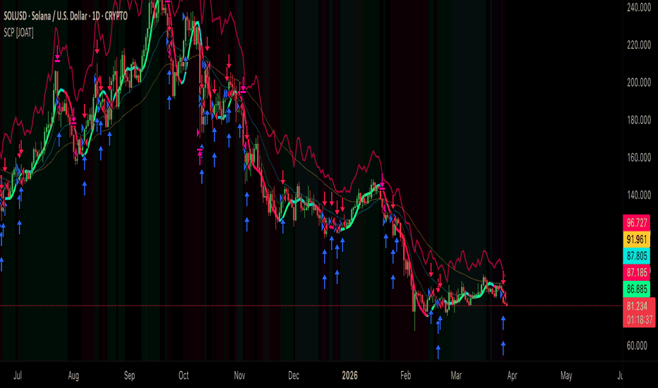
Phantom Whale Hunter [JOAT]Phantom Whale Hunter
Introduction
The Phantom Whale Hunter is an advanced open-source institutional footprint tracking system that combines Chaikin Money Flow, Money Flow Index, On-Balance Volume, VWAP analysis, and Accumulation/Distribution to detect institutional buying and selling pressure. This indicator reveals when large institutional players (whales) are accumulating or distributing positions, providing traders with insights into smart money positioning before major price moves occur.
Unlike basic volume indicators, the Phantom Whale Hunter provides multi-dimensional institutional flow analysis through money flow calculations, volume-weighted analysis, cumulative volume tracking, and phase detection. The indicator is designed for traders who understand that institutional money moves markets and that detecting whale footprints early provides significant trading advantages.
Why This Indicator Exists
This indicator addresses the need for systematic institutional flow analysis. By combining five distinct money flow methodologies with phase detection, it reveals:
Chaikin Money Flow (CMF): Measures buying/selling pressure based on close position within range
Money Flow Index (MFI): Volume-weighted RSI showing money flow strength
On-Balance Volume (OBV): Cumulative volume indicator tracking institutional accumulation/distribution
VWAP Analysis: Volume-weighted average price with deviation bands
Accumulation/Distribution (A/D): Cumulative indicator measuring money flow into/out of security
Institutional Flow Index: Composite measure combining all five components
Phase Detection: Classifies market as Strong Accumulation, Accumulation, Neutral, Distribution, or Strong Distribution
Smart Money Divergence: Detects when price and flow move in opposite directions
Core Components Explained
1. Chaikin Money Flow (CMF)
CMF measures the relationship between close position and volume:
Money Flow Volume: ((Close - Low) - (High - Close)) / (High - Low) × Volume
CMF Calculation: Sum of MFV over period / Sum of volume over period
CMF Smoothing: 7-period EMA for noise reduction
Interpretation: CMF > 0 = buying pressure, CMF < 0 = selling pressure
CMF values above +0.1 indicate strong buying pressure, while values below -0.1 indicate strong selling pressure.
2. Money Flow Index (MFI)
MFI is a volume-weighted momentum indicator:
Typical Price: (High + Low + Close) / 3
Raw Money Flow: Typical Price × Volume
Positive Flow: Money flow when typical price rises
Negative Flow: Money flow when typical price falls
Money Ratio: Sum of positive flow / Sum of negative flow
MFI: 100 - (100 / (1 + Money Ratio))
MFI above 80 indicates overbought with high volume (potential distribution), while MFI below 20 indicates oversold with high volume (potential accumulation).
3. On-Balance Volume (OBV)
OBV tracks cumulative volume flow:
Calculation: Add volume on up days, subtract volume on down days
Cumulative: Running total from start of data
Normalization: Scaled to 0-100 range using 100-bar high/low
Zero-Centering: Subtract 50 for composite integration
Rising OBV with rising price confirms uptrend (accumulation). Falling OBV with rising price warns of distribution.
4. VWAP (Volume-Weighted Average Price)
VWAP calculates the average price weighted by volume:
Calculation: Sum(Typical Price × Volume) / Sum(Volume)
Daily Reset: VWAP resets at start of each trading day
Standard Deviation: Measures price dispersion from VWAP
Deviation Bands: VWAP ± (StdDev × Multiplier)
Price vs VWAP: Percentage distance from VWAP
Price above VWAP indicates bullish institutional positioning. Price below VWAP indicates bearish institutional positioning. Large deviations often mean-revert.
5. Accumulation/Distribution (A/D) Line
A/D measures cumulative money flow:
Money Flow Multiplier: ((Close - Low) - (High - Close)) / (High - Low)
Money Flow Volume: Multiplier × Volume
A/D Line: Cumulative sum of money flow volume
Smoothing: EMA smoothing (default 14) for trend identification
Normalization: Scaled to 0-100 range, then zero-centered
Rising A/D with rising price confirms accumulation. Falling A/D with rising price signals distribution (bearish divergence).
6. Institutional Flow Index Calculation
All five components are combined into a unified flow index:
Flow Index = (CMF × 50 + (MFI - 50) + (OBV - 50) + (A/D - 50)) / 4
This composite index ranges from approximately -50 to +50, with:
Flow Index > 30 = Strong institutional buying
Flow Index > 10 = Institutional buying
Flow Index -10 to +10 = Neutral/balanced
Flow Index < -10 = Institutional selling
Flow Index < -30 = Strong institutional selling
7. Phase Detection System
The indicator classifies institutional positioning into five phases:
Strong Accumulation (Phase 2): Flow Index > 30, CMF > 0.1, MFI > 50
Accumulation (Phase 1): Flow Index > 10, CMF > 0
Neutral (Phase 0): Flow Index between -10 and +10
Distribution (Phase -1): Flow Index < -10, CMF < 0
Strong Distribution (Phase -2): Flow Index < -30, CMF < -0.1, MFI < 50
Phase classification helps identify when institutions are actively positioning.
8. Smart Money Divergence Detection
Divergences occur when price and flow move in opposite directions:
Price Momentum: 14-period rate of change in price
Flow Momentum: 14-period rate of change in Flow Index
Bullish Divergence: Price falling (momentum < 0), Flow rising (momentum > 0)
Bearish Divergence: Price rising (momentum > 0), Flow falling (momentum < 0)
Smart money divergences indicate institutions positioning against current price trend, often preceding reversals.
9. Institutional Pressure Detection
The indicator identifies strong institutional buying/selling:
Buy Pressure: CMF > 0, MFI > 50, OBV > 50, Volume Surge
Sell Pressure: CMF < 0, MFI < 50, OBV < 50, Volume Surge
Volume Surge: Current volume > average volume × 2.25
Anti-Overlap: Minimum 25 bars between pressure signals
Institutional pressure with volume confirmation indicates significant whale activity.
10. Flow Velocity and Acceleration
The indicator tracks flow momentum:
Flow Velocity: Change in Flow Index (first derivative)
Flow Acceleration: Change in velocity (second derivative)
Accelerating flow indicates increasing institutional participation. Decelerating flow warns of waning institutional interest.
Visual Elements
Institutional Flow Line: Main line showing composite flow with phase-based coloring (green = accumulation, red = distribution, yellow = neutral)
Component Lines: Four thin lines showing CMF, MFI, OBV, and A/D (all normalized)
Zero Line: Horizontal line at zero
Threshold Lines: Dashed lines at +30 (strong accumulation), +10 (accumulation), -10 (distribution), -30 (strong distribution)
Zone Fills: Shaded areas above +30 (green) and below -30 (red)
Volume Surge Background: Purple background when volume surges occur
Smart Money Divergence Circles: Small circles marking divergence points
Institutional Pressure Triangles: Triangles marking strong buy/sell pressure
Flow Velocity Histogram: Shows rate of change in flow
Information Dashboard: Displays phase, flow index, CMF, MFI, OBV, A/D, volume ratio, price vs VWAP, flow velocity, and signal status
How to Use This Indicator
Step 1: Check Current Phase
Monitor the dashboard for institutional phase (Strong Accumulation, Accumulation, Neutral, Distribution, Strong Distribution).
Step 2: Analyze Flow Index
Flow Index > 20 = institutional buying, Flow Index < -20 = institutional selling. Trade in direction of institutional flow.
Step 3: Confirm with Components
Check CMF, MFI, OBV, and A/D for confirmation. All four positive = strongest accumulation signal.
Step 4: Monitor Volume Ratio
Volume surges (> 2x average) with positive flow confirm institutional buying. Volume surges with negative flow confirm institutional selling.
Step 5: Check Price vs VWAP
Price above VWAP with positive flow = bullish institutional positioning. Price below VWAP with negative flow = bearish institutional positioning.
Step 6: Watch for Smart Money Divergences
Divergences at extreme flow levels often precede reversals. Purple circles mark these critical points.
Step 7: Look for Institutional Pressure
Triangles mark strong institutional buy/sell pressure with volume confirmation. These are high-probability signals.
Best Practices
Trade in direction of institutional phase - don't fight whale positioning
Wait for Strong Accumulation/Distribution phases for highest conviction
Confirm flow signals with volume surges - flow without volume may be weak
Use smart money divergences as early reversal warnings
Monitor flow velocity - accelerating flow indicates increasing institutional participation
Combine with price action and support/resistance for entry timing
Be patient - institutional accumulation/distribution can take time
Use higher timeframe flow for stronger significance
Input Parameters
Chaikin Money Flow:
CMF Length: Period for CMF calculation (default: 20)
Money Flow Index:
MFI Length: Period for MFI calculation (default: 14)
MFI Overbought: Threshold for overbought (default: 80)
MFI Oversold: Threshold for oversold (default: 20)
Volume Configuration:
Volume MA Length: Period for average volume (default: 20)
Surge Threshold: Multiplier for volume surges (default: 2.0x)
Show Volume Profile: Toggle volume display (default: enabled)
VWAP Analysis:
VWAP Std Dev: Standard deviation multiplier (default: 2.0)
Accumulation/Distribution:
A/D Smoothing: EMA smoothing period (default: 14)
Phase Threshold: Threshold for phase classification (default: 0.5)
Visual Configuration:
Accumulation/Distribution/Neutral/Smart Money Colors: Customizable colors
Originality Statement
This indicator is original in its comprehensive institutional flow approach. While individual components (CMF, MFI, OBV, VWAP, A/D) are established concepts, this indicator is justified because:
It combines five distinct money flow methodologies into a unified institutional flow index
The phase detection system classifies institutional positioning systematically
Smart money divergence detection identifies when institutions position against price
Institutional pressure detection with volume confirmation reveals whale activity
Flow velocity and acceleration tracking predict institutional momentum changes
Integration of VWAP analysis provides institutional price positioning context
The comprehensive dashboard presents all institutional flow metrics simultaneously
Disclaimer
This indicator is provided for educational and informational purposes only. It is not financial advice. Trading involves substantial risk of loss. Institutional flow analysis does not guarantee profitable trades. Whale activity does not guarantee price direction. Always use proper risk management and never risk more than you can afford to lose.
-Made with passion by officialjackofalltrades インジケーター

Turbulence Fractal Scanner [JOAT]Turbulence Fractal Scanner
Introduction
The Turbulence Fractal Scanner is an advanced open-source volatility chaos prediction engine that combines ATR, Bollinger Band Width, Keltner Channels, Historical Volatility, and Squeeze detection into a unified volatility analysis system. This indicator measures market turbulence across multiple dimensions, creating a comprehensive volatility index that reveals expansion/contraction cycles, squeeze conditions, and breakout predictions.
Unlike single-dimension volatility indicators, the Turbulence Fractal Scanner provides multi-layered volatility intelligence through percentile ranking, composite indexing, regime classification, and squeeze detection. The indicator is designed for traders who understand that volatility precedes price movement and that multi-dimensional volatility analysis provides early warning of significant market shifts.
Why This Indicator Exists
This indicator addresses the need for comprehensive volatility analysis that goes beyond simple ATR or Bollinger Bands. By combining five distinct volatility methodologies, it reveals:
ATR Analysis: Average True Range measures actual price movement volatility
Bollinger Band Width: Measures price dispersion relative to moving average
Keltner Channels: ATR-based bands for volatility envelope detection
Historical Volatility: Statistical measure of price returns volatility
Squeeze Detection: Identifies when Bollinger Bands contract inside Keltner Channels
Composite Volatility Index: Unified measure combining all five components
Regime Classification: Categorizes volatility as Low, Normal, High, or Squeeze
Breakout Prediction: Detects squeeze breakouts with directional bias
Core Components Explained
1. ATR (Average True Range) Analysis
ATR measures the average range of price movement:
True Range: Maximum of (high - low), (high - previous close), (previous close - low)
ATR Calculation: Moving average of true range over period (default 14)
ATR Smoothing: Additional EMA smoothing (default 7) reduces noise
ATR Percent: ATR divided by close, expressed as percentage
ATR Percentile: ATR ranked against 100-bar history (0-100 scale)
ATR percentile shows whether current volatility is high or low relative to recent history. High percentile (> 70) indicates elevated volatility, low percentile (< 30) indicates compressed volatility.
2. Bollinger Band Width Analysis
BB Width measures price dispersion:
Bollinger Bands: SMA ± (standard deviation × multiplier)
BB Width: (Upper band - Lower band) / Middle band × 100
BB Width Percentile: Current width ranked against 100-bar history
Narrow BB Width indicates low volatility and potential breakout setup. Wide BB Width indicates high volatility and potential mean reversion.
3. Keltner Channel Analysis
Keltner Channels use ATR for volatility bands:
Basis: EMA of close (default 20 periods)
Range: ATR × multiplier (default 1.5)
Upper/Lower: Basis ± Range
Keltner Channels adapt to volatility changes and are used in squeeze detection.
4. Squeeze Detection
Squeeze occurs when Bollinger Bands contract inside Keltner Channels:
Squeeze On: BB Lower > KC Lower AND BB Upper < KC Upper
Squeeze Off: Bands no longer contracted
Squeeze Breakout: Transition from Squeeze On to Squeeze Off
Breakout Direction: Determined by close comparison (close > close = bullish)
Squeezes indicate extreme volatility compression. Breakouts from squeezes often lead to significant directional moves.
5. Historical Volatility (HV) Calculation
HV measures statistical volatility of returns:
Returns: Logarithmic price changes (log(close / close ))
Standard Deviation: StdDev of returns over period (default 20)
Annualization: Multiply by sqrt(252) for annual volatility (optional)
HV Percentile: Current HV ranked against 100-bar history
HV provides a statistical measure of actual price volatility, complementing the technical measures (ATR, BB Width).
6. Composite Volatility Index
All three percentile measures are combined into a unified index:
Volatility Index = (ATR Percentile + BB Width Percentile + HV Percentile) / 3
This composite index provides a balanced view of volatility across multiple methodologies. Values range from 0 (extremely low volatility) to 100 (extremely high volatility).
7. Volatility Regime Classification
The indicator classifies volatility into four regimes:
Squeeze (Priority): When squeeze is active, regardless of volatility index
Low Volatility: Volatility Index < threshold (default 30)
Normal Volatility: Volatility Index between low and high thresholds (30-70)
High Volatility: Volatility Index > threshold (default 70)
Regime classification helps traders adapt strategies to current volatility conditions.
8. Volatility Trend Analysis
The indicator tracks volatility direction:
Volatility Trend: 5-period SMA of Volatility Index
Rising Volatility: Trend rising for 3+ consecutive bars
Falling Volatility: Trend falling for 3+ consecutive bars
Expansion: Volatility Index rising for 3+ consecutive bars
Contraction: Volatility Index falling for 3+ consecutive bars
Volatility trends help predict whether turbulence is increasing or decreasing.
9. Breakout Prediction System
The indicator predicts breakouts from squeeze conditions:
Squeeze Breakout: Detected when squeeze transitions from On to Off
Direction: Bullish if close > close , bearish if close < close
Volatility Confirmation: Best breakouts occur when Volatility Index < 40 (compressed)
Breakouts from low volatility squeezes often lead to sustained directional moves.
10. Turbulence Shift Detection
The indicator identifies regime changes:
Regime Shift: When volatility regime changes (Low ↔ Normal ↔ High ↔ Squeeze)
Anti-Overlap: Minimum 10 bars between shift signals
High Vol Entry: Shift into High Volatility regime
Low Vol Entry: Shift into Low Volatility regime
Regime shifts provide early warning of changing market conditions.
Visual Elements
Volatility Index Line: Main line showing composite volatility with regime-based coloring (purple = squeeze, red = high, cyan = low, yellow = normal)
Component Lines: Three thin lines showing ATR, BB Width, and HV percentiles
Volatility Trend Line: Step-line showing smoothed volatility trend
Threshold Lines: Horizontal lines at high (70) and low (30) thresholds, plus median (50)
Zone Fills: Shaded areas above high threshold (red) and below low threshold (cyan)
Squeeze Background: Purple background when squeeze is active
Breakout Signals: Triangles marking squeeze breakouts (cyan = bullish, red/orange = bearish)
Regime Shift Circles: Small circles marking regime transitions
Information Dashboard: Displays regime, volatility index, ATR/BB/HV percentiles, squeeze status, volatility trend, expansion/contraction, breakout status, ATR/BB values, and overall signal
How to Use This Indicator
Step 1: Check Volatility Regime
Monitor the dashboard for current regime (Squeeze, Low Vol, Normal, High Vol). Adapt strategy to regime.
Step 2: Monitor Volatility Index
Volatility Index < 30 = compressed (potential breakout setup)
Volatility Index > 70 = elevated (potential mean reversion or continuation)
Step 3: Watch for Squeeze Conditions
Purple background indicates squeeze. Prepare for breakout when squeeze ends.
Step 4: Identify Breakout Direction
When squeeze breakout occurs, triangle color shows direction (cyan = bullish, red = bearish).
Step 5: Check Volatility Trend
Rising volatility = increasing turbulence, falling volatility = calming conditions.
Step 6: Monitor Expansion/Contraction
Expanding volatility often precedes strong moves. Contracting volatility suggests consolidation.
Step 7: Use Regime Shifts as Alerts
Shifts into High Vol or Low Vol regimes provide early warning of changing conditions.
Best Practices
Trade breakouts from squeeze conditions with low volatility index (< 40)
Avoid trend-following strategies in high volatility regimes (> 70)
Use low volatility regimes (< 30) to prepare for breakout setups
Monitor all three components (ATR, BB, HV) for confirmation
Rising volatility in low regime warns of impending breakout
Falling volatility in high regime suggests consolidation ahead
Combine with trend indicators - volatility shows when, trend shows direction
Be cautious of false breakouts - wait for volatility confirmation
Input Parameters
ATR Configuration:
ATR Length: Period for ATR calculation (default: 14)
ATR Smoothing: EMA smoothing period (default: 7)
Bollinger Bands:
BB Length: Period for BB calculation (default: 20)
BB Multiplier: Standard deviation multiplier (default: 2.0)
Keltner Channels:
KC Length: Period for KC basis (default: 20)
KC Multiplier: ATR multiplier for bands (default: 1.5)
Historical Volatility:
HV Length: Period for HV calculation (default: 20)
Annualize HV: Convert to annual volatility (default: enabled)
Regime Thresholds:
Low Volatility: Threshold for low regime (default: 30)
High Volatility: Threshold for high regime (default: 70)
Visual Configuration:
Low/Normal/High/Squeeze Colors: Customizable regime colors
Originality Statement
This indicator is original in its comprehensive volatility analysis approach. While individual components (ATR, BB, KC, HV, Squeeze) are established concepts, this indicator is justified because:
It combines five distinct volatility methodologies into a unified composite index
Percentile ranking normalizes all components to a common 0-100 scale
The regime classification system categorizes volatility conditions systematically
Squeeze detection with breakout prediction provides actionable trading signals
Volatility trend and expansion/contraction analysis predict volatility direction
Turbulence shift detection identifies regime changes early
The comprehensive dashboard presents all volatility dimensions simultaneously
Disclaimer
This indicator is provided for educational and informational purposes only. It is not financial advice. Trading involves substantial risk of loss. Volatility analysis does not guarantee profitable trades. Low volatility does not guarantee breakouts. High volatility does not guarantee reversals. Always use proper risk management and never risk more than you can afford to lose.
-Made with passion by officialjackofalltrades インジケーター

Divergence Constellation [JOAT]Divergence Constellation
Introduction
The Divergence Constellation is an advanced open-source multi-oscillator divergence detection system that combines RSI, MACD, TSI, and Stochastic analysis with sophisticated pivot detection and confluence scoring. This indicator identifies both regular and hidden divergences across multiple oscillators simultaneously, creating a constellation of divergence signals that reveal potential reversals and trend continuations with high probability.
Unlike single-oscillator divergence tools, the Divergence Constellation provides multi-dimensional divergence analysis through composite oscillator calculation, four-oscillator confluence scoring, regular and hidden divergence detection, and chart projection. The indicator is designed for traders who understand that divergences confirmed across multiple oscillators provide significantly higher probability setups than single-oscillator divergences.
Why This Indicator Exists
This indicator addresses the need for systematic multi-oscillator divergence analysis. By combining four distinct oscillators with confluence scoring, it reveals:
Regular Bullish Divergence: Price makes lower low, oscillators make higher low (reversal up signal)
Regular Bearish Divergence: Price makes higher high, oscillators make lower high (reversal down signal)
Hidden Bullish Divergence: Price makes higher low, oscillators make lower low (trend continuation up)
Hidden Bearish Divergence: Price makes lower high, oscillators make higher high (trend continuation down)
Confluence Scoring: Counts how many oscillators confirm the divergence (1-4 score)
Composite Oscillator: Unified oscillator combining all four components
Chart Projection: Divergence lines drawn on both oscillator pane and main chart
Core Components Explained
1. Four-Oscillator System
The indicator calculates four distinct oscillators, each providing unique momentum perspective:
RSI (Relative Strength Index):
Measures momentum by comparing average gains to average losses
Zero-centered (subtracts 50) for composite integration
Sensitive to overbought/oversold conditions
Default period: 14
MACD (Moving Average Convergence Divergence):
Measures relationship between two exponential moving averages
Histogram shows momentum acceleration/deceleration
Responsive to trend changes
Default periods: 12, 26, 9
TSI (True Strength Index):
Double-smoothed momentum indicator
Filters noise while preserving trend direction
Excellent for divergence detection
Default periods: 25, 13
Stochastic:
Compares close to recent high-low range
Zero-centered (subtracts 50) for composite integration
Identifies overbought/oversold extremes
Default periods: 14, 3
2. Composite Oscillator Calculation
All four oscillators are combined into a unified composite:
Composite = (RSI + MACD + TSI + Stochastic) / 4
This composite oscillator provides a balanced view of momentum across all four methodologies. Divergences are detected on the composite, then confirmed by checking individual oscillators.
3. Pivot Detection System
The indicator uses sophisticated pivot detection to identify divergence points:
Pivot Left/Right: Number of bars on each side for pivot confirmation (default: 5)
Price Pivots: Identifies swing highs and lows in price
Oscillator Pivots: Identifies swing highs and lows in each oscillator
Lookback Range: Min (5) to Max (60) bars for comparing pivots
Pivots must be confirmed (bars on both sides) before divergence analysis begins.
4. Regular Divergence Detection
Regular divergences signal potential reversals:
Regular Bullish Divergence:
Price makes lower low (current pivot low < previous pivot low)
Composite oscillator makes higher low (current pivot low > previous pivot low)
Indicates weakening downward momentum - potential reversal up
Best at oversold levels (composite < -20)
Regular Bearish Divergence:
Price makes higher high (current pivot high > previous pivot high)
Composite oscillator makes lower high (current pivot high < previous pivot high)
Indicates weakening upward momentum - potential reversal down
Best at overbought levels (composite > 20)
5. Hidden Divergence Detection
Hidden divergences signal trend continuation:
Hidden Bullish Divergence:
Price makes higher low (current pivot low > previous pivot low)
Composite oscillator makes lower low (current pivot low < previous pivot low)
Indicates strong underlying bullish momentum - trend continuation up
Confirms uptrend strength
Hidden Bearish Divergence:
Price makes lower high (current pivot high < previous pivot high)
Composite oscillator makes higher high (current pivot high > previous pivot high)
Indicates strong underlying bearish momentum - trend continuation down
Confirms downtrend strength
6. Confluence Scoring System
When a divergence is detected on the composite, the indicator checks all four individual oscillators:
Score 1/4: Only one oscillator confirms - weak divergence
Score 2/4: Two oscillators confirm - moderate divergence (minimum for signals)
Score 3/4: Three oscillators confirm - strong divergence
Score 4/4: All four oscillators confirm - extreme divergence (highest probability)
The minimum confluence score (default 2) filters out weak divergences that lack multi-oscillator confirmation.
7. Signal Generation Logic
Signals are generated only at extreme oscillator levels with anti-overlap logic:
Bullish Signals:
Regular bullish divergence detected
Composite oscillator < -20 (oversold)
Confluence score >= minimum (default 2)
At least 20 bars since last bullish signal (anti-overlap)
Bearish Signals:
Regular bearish divergence detected
Composite oscillator > 20 (overbought)
Confluence score >= minimum (default 2)
At least 20 bars since last bearish signal (anti-overlap)
Extreme Signals:
Confluence score = 4/4 (all oscillators confirm)
Composite at extreme levels (< -30 or > 30)
Displayed as diamond shapes for emphasis
8. Visual Divergence Lines
Divergence lines are drawn connecting pivot points:
Regular Divergences: Solid lines (green = bullish, red = bearish)
Hidden Divergences: Dashed lines (cyan = bullish, orange = bearish)
Oscillator Pane: Lines drawn on composite oscillator
Chart Projection: Lines also drawn on main price chart (optional)
Lines provide visual confirmation of the divergence pattern and help identify the exact pivot points involved.
Visual Elements
Four Oscillator Lines: Thick colored lines showing RSI (cyan), MACD (magenta), TSI (yellow), and Stochastic (green)
Composite Line: White line showing unified oscillator
Zero Line: Gray horizontal line at zero
Overbought/Oversold Zones: Shaded areas at +30/-30 levels
Divergence Lines: Solid/dashed lines connecting pivot points
Signal Triangles: Small triangles at signal generation points
Extreme Diamonds: Larger diamonds for 4/4 confluence signals
Information Dashboard: Displays composite position, confluence score, RSI/MACD/TSI/Stochastic status, composite value, divergence types, signal strength, extreme events, and overall verdict
How to Use This Indicator
Step 1: Monitor Composite Position
Check if composite oscillator is at extreme levels (> 30 overbought, < -30 oversold). Divergences at extremes have highest probability.
Step 2: Check Confluence Score
Look for confluence scores of 3/4 or 4/4. Higher scores indicate stronger divergence confirmation across multiple oscillators.
Step 3: Identify Divergence Type
Regular divergences signal reversals, hidden divergences signal trend continuation. Trade accordingly.
Step 4: Wait for Signal Confirmation
Don't trade divergence lines alone. Wait for signal triangles that confirm divergence meets all criteria (extreme level, confluence, anti-overlap).
Step 5: Look for Extreme Events
Diamond shapes indicate 4/4 confluence at extreme levels - highest probability setups.
Step 6: Confirm with Price Action
Use divergence signals as alerts, then confirm with price action, support/resistance, or other indicators before entering.
Step 7: Check Individual Oscillators
Dashboard shows status of each oscillator. All four overbought/oversold provides additional confirmation.
Best Practices
Trade only divergences with confluence score >= 2 (default minimum)
Focus on regular divergences at extreme levels (< -30 or > 30) for reversals
Use hidden divergences to confirm trend continuation, not as standalone entries
Wait for signal triangles - don't front-run divergence lines
4/4 confluence signals (diamonds) offer highest probability setups
Combine with support/resistance levels for additional confirmation
Avoid divergences in middle range (-20 to +20) - wait for extremes
Use higher timeframe divergences for stronger significance
Input Parameters
Pivot Detection:
Pivot Left: Bars to left of pivot (default: 5)
Pivot Right: Bars to right of pivot (default: 5)
Max Lookback: Maximum bars to compare pivots (default: 60)
Min Lookback: Minimum bars to compare pivots (default: 5)
Oscillator Configuration:
RSI Length: Period for RSI (default: 14)
MACD Fast: Fast EMA period (default: 12)
MACD Slow: Slow EMA period (default: 26)
MACD Signal: Signal line period (default: 9)
TSI Long: Long smoothing period (default: 25)
TSI Short: Short smoothing period (default: 13)
Stochastic K: K period (default: 14)
Stochastic D: D smoothing (default: 3)
Divergence Rules:
Show Regular Divergence: Toggle regular divergence detection (default: enabled)
Show Hidden Divergence: Toggle hidden divergence detection (default: enabled)
Min Confluence Score: Minimum oscillators that must confirm (default: 2)
Project on Chart: Draw divergence lines on main chart (default: enabled)
Visual Configuration:
Bullish/Bearish Divergence Colors: Colors for regular divergences
Hidden Bullish/Bearish Colors: Colors for hidden divergences
Originality Statement
This indicator is original in its multi-oscillator confluence approach. While individual oscillators and divergence concepts are established, this indicator is justified because:
It combines four distinct oscillators into a unified composite system
The confluence scoring system measures divergence strength across multiple oscillators
Automatic detection of both regular and hidden divergences with pivot analysis
Signal generation includes extreme level filtering and anti-overlap logic
Chart projection allows divergence visualization on both oscillator and price chart
The comprehensive dashboard presents all oscillator states and divergence metrics simultaneously
Integration of multiple oscillator perspectives creates higher probability divergence signals
Disclaimer
This indicator is provided for educational and informational purposes only. It is not financial advice. Trading involves substantial risk of loss. Divergence analysis does not guarantee profitable trades or reversals. Past divergences do not guarantee future results. Always use proper risk management and never risk more than you can afford to lose.
-Made with passion by officialjackofalltrades インジケーター

Elliott Wave Detector PRO [TGTBTB]Elliott Wave Advanced v3 — Validated Wave Counting with Pattern Detection
A word before you start
Elliott Wave is supposedly one of the most powerful frameworks in technical analysis — and also one of the most difficult to apply correctly. The theory involves layers of rules, guidelines, pattern variations, and degree relationships that even experienced practitioners argue about. Automating it is genuinely hard, and no indicator (including this one) will get every count right every time. I felt like banging my head onto my desk more than once while trying to translate the rules into code....
What I tried to do here is capture the core rules and guidelines as faithfully as possible and make them accessible in a way that keeps things honest. The indicator won't show you a wave count unless it actually passes validation. That means you'll sometimes stare at a chart full of dot markers with no labels — and that's a feature, not a bug. I'd rather tell you "I don't know" than confidently show you something wrong.
I've put serious effort into getting the rule enforcement, pattern detection, and Fibonacci relationships right, but Elliott Wave will always involve interpretation. Treat this as a tool that tries to take the objective parts of the theory off your shoulders so you can focus on the parts that require judgment.
I deliberately made this indicator open source because I am not an Elliott Wave expert. So if you notice anything that is absolutely wrong according to the rulebook of Elliott Wave leave a message below or contact me directly so I can bug fix this indicator. The goal is to make Elliott Wave theory accessible to everyone.
What differentiates this indicator from other Elliot Wave indicators
This indicator attempts to solve the biggest problem with Elliott Wave analysis on charts: most auto-labelers just slap wave numbers onto every swing without checking if the count is actually valid.
Elliott Wave theory has three rules that cannot be broken. Ever. If your wave count violates any of them, it's wrong — no discussion. This indicator enforces all three before putting a single label on your chart:
1. Wave 2 never retraces beyond the start of Wave 1
2. Wave 3 is never the shortest among waves 1, 3, and 5
3. Wave 4 does not enter Wave 1's price territory (unless it's a diagonal)
If the pivots on your chart don't satisfy these rules, you won't see wave numbers — you'll see neutral dot markers instead. That's intentional. I'd rather show you nothing than show you a wrong count. Too many indicators out there label every zig-zag as "wave 3" and give people false confidence. This one stays quiet when it's not sure.
Pattern Detection
The indicator identifies five pattern types:
Impulse (5-wave motive) — Five alternating swings validated against all three cardinal rules, with confidence scoring based on Fibonacci proportions between the waves. Wave 3 at 1.618x Wave 1 - a high-confidence impulse. Wave 3 barely longer than Wave 1? Still valid, but lower confidence, which gets reflected by the score
Diagonal (Leading / Ending) — Same five-wave structure, but with the key difference that Wave 4 overlaps Wave 1. The indicator checks for a converging wedge shape and progressively shorter waves. These show up at the start or end of larger wave sequences and are easy to miscount as impulses if you're not checking for overlap.
Zigzag (A-B-C sharp correction) — Three-wave correction where Wave B typically retraces 38-79% of Wave A, and Wave C often equals Wave A in length. The indicator validates B doesn't exceed A's origin and C reaches beyond A's end.
Flat (Regular & Expanded) — Wave B retraces almost all of Wave A (or exceeds it in an expanded flat), and Wave C approximates Wave A's length. The indicator distinguishes between regular flats (B ≈ 100% of A) and expanded flats (B > 105% of A) because they have different trading implications.
Contracting Triangle (A-B-C-D-E) — Five-wave sideways pattern with converging boundaries. Each successive wave should be shorter than the previous one. The indicator checks that highs are declining and lows are rising, and requires at least 3 out of 4 contraction relationships to hold (real markets aren't always perfectly geometric).
Guidelines
Elliott Wave has rules (hard constraints) and guidelines (soft constraints that affect probability). This indicator checks both of them:
Alternation — If Wave 2 is a sharp, deep correction, Wave 4 should be a shallow, sideways one, and vice versa. The indicator classifies each correction based on retracement depth and duration relative to the preceding impulse, then checks whether waves 2 and 4 have different character. This isn't a dealbreaker if it fails, but it affects the confidence score and is shown on the info panel (✓ or ✗).
Sub-wave structure — Motive waves (1, 3, 5) should subdivide into 5 sub-waves internally, while corrective waves (2, 4) should subdivide into 3. The indicator counts secondary pivots within each primary wave's time range and checks if the internal structure is consistent with what Elliott Wave theory expects. Again, not a hard gate, but it influences confidence scoring.
Fibonacci Analysis
The Fibonacci levels are calculated with proper anchor points:
Retracements are projected from the last completed wave — showing where the current correction might find support/resistance.
Extensions use the correct Elliott Wave method: the prior impulse wave's length is projected from the corrective wave's end. So if you've completed waves 1-2, the Wave 3 target is projected as a 1.618 extension of Wave 1's length measured from Wave 2's end. Not from some arbitrary reference point.
When a validated pattern exists, the extension anchors are taken directly from the identified wave structure. When there's no confirmed pattern, it falls back to geometric pivot-based projection (and tells you so).
The Forecast Panel
I made a deliberate design choice for this: the forecast is gated behind pattern confirmation.
If the indicator has identified a validated impulse, zigzag, flat, triangle, or diagonal, the forecast panel shows "CONFIRMED" and provides wave-structure-aware targets and scenarios. After a completed correction, it projects the next impulse in the correct direction. After a completed impulse, it anticipates the corrective phase.
If no pattern has been validated, the forecast shows "UNCONFIRMED" and limits itself to cautious directional observations based on raw pivot geometry. No wave labels, no "Wave 3 starting!" claims, but a honest reporting of what the price structure looks like without pretending to know more than it does.
The projection lines on the chart reflect this too — confirmed forecasts get solid, visible projections; unconfirmed ones are thinner and more transparent.
Trade Signals
Three signal types, all requiring some degree of pattern confirmation:
-Wave 3 Entry — Fires after a valid Wave 2 retracement (38.2-78.6%) when the indicator has at least moderate confidence in the count
- Wave 5 Exit — Triggers when momentum is waning in a confirmed impulse (last wave significantly shorter than the overall move)
- Wave C Reversal — Signals when a validated zigzag or flat correction is complete and the reversal should begin
Signals won't fire on an unconfirmed wave count. If the indicator isn't sure what wave you're in, it won't pretend to give you entries.
Settings & Tuning
Swing Detection — The two most important inputs. "Primary Wave Swing Length" controls how many bars are needed to confirm a major swing (lower = more sensitive, more pivots, more patterns detected but potentially noisier). "Min Swing %" sets the minimum percentage move to qualify as a primary wave — for crypto on daily timeframes, 5-10% works well. For forex or equities you'll want to bring this down.
Sub-Wave Swing Length — Controls the secondary pivot detection used for internal structure validation. Keep this lower than the primary setting.
Everything else in the settings is display-related and fairly self-explanatory. Colors, text sizes, which elements to show/hide.
What this is NOT
This is not a crystal ball. Elliott Wave analysis is inherently subjective — two analysts can look at the same chart and produce different valid counts. What this indicator does is enforce the objective constraints of the theory and give you a probabilistic assessment of which pattern best fits the current structure.
It works best on higher timeframes (4H, Daily, Weekly) where the swing structure is cleaner. On 1-minute charts you'll mostly see dot markers because the noise rarely resolves into validated patterns — and that's the indicator doing its job correctly.
Use it alongside your other analysis. The wave count gives you context for where you are in the cycle. The Fibonacci levels give you targets. The signals give you timing. But none of it replaces risk management and position sizing. インジケーター

Velocity Spectrum Analyzer [JOAT]Velocity Spectrum Analyzer
Introduction
The Velocity Spectrum Analyzer is an advanced open-source momentum wave system that combines Munich Wave methodology with ALMA enhancement and multi-basis momentum tracking. This indicator analyzes momentum across five distinct velocity layers, creating a spectrum of momentum waves that reveal trend strength, regime shifts, and momentum alignment across multiple timeframes.
Unlike single-line momentum indicators, the Velocity Spectrum Analyzer provides multi-dimensional momentum analysis through layered EMA calculations, ALMA enhancement, regime classification, and spread analysis. The indicator is designed for traders who understand that momentum flows in waves and that multi-layer alignment signals institutional conviction.
Why This Indicator Exists
This indicator addresses the need for multi-dimensional momentum analysis. By combining five momentum layers with ALMA enhancement and regime detection, it reveals:
Five Velocity Layers: Fast (9), Medium (21), Slow (55), Very Slow (100), and Ultra Slow (200) EMAs create a momentum spectrum
ALMA Enhancement: Arnaud Legoux Moving Average provides adaptive smoothing with reduced lag
Basis Calculations: Averages between EMA layers create intermediate momentum levels
Regime Classification: Extreme Bull/Bear detection using Bollinger-style bands
Spread Analysis: Distance between fast and slow layers measures momentum strength
Wave State Detection: All layers bullish or bearish signals strong directional momentum
Background Coloring: Visual regime indication shows extreme conditions
Core Components Explained
1. Core Momentum Calculation
The indicator starts with basic momentum (current close minus close N bars ago), then applies ALMA for adaptive smoothing:
The ALMA offset (default 0.85) and sigma (default 6) parameters control the balance between responsiveness and smoothness. Higher offset values shift the average toward recent prices, while higher sigma values increase smoothness.
2. Five EMA Layers
Five EMAs are calculated on the momentum values:
Fast EMA (9): Captures short-term momentum shifts
Medium EMA (21): Tracks intermediate momentum trends
Slow EMA (55): Identifies primary momentum direction
Very Slow EMA (100): Reveals long-term momentum bias
Ultra Slow EMA (200): Shows institutional momentum positioning
Each layer responds at different speeds, creating a spectrum of momentum perspectives.
3. Basis Calculations
Five basis levels are calculated as averages between EMA layers:
Basis 1: Average of Fast and Medium EMAs
Basis 2: Average of Medium and Slow EMAs
Basis 3: Average of Slow and Very Slow EMAs
Basis 4: Average of Very Slow and Ultra Slow EMAs
Basis 5: Average of Ultra Slow and Fast EMAs (wraps around)
These basis levels create intermediate momentum zones that smooth transitions between layers.
4. Trend Classification Functions
Two functions classify momentum direction:
Growing: Momentum > basis (bullish momentum)
Falling: Momentum <= basis AND momentum <= ALMA (bearish momentum)
Each basis is classified independently, creating five separate momentum assessments.
5. Regime Detection with Bollinger-Style Bands
The indicator calculates bands around the average of all five basis levels:
Origin: SMA of basis average (default 25 periods)
Deviation: Standard deviation multiplied by factor (default 6.0)
Top Band: Origin + deviation (extreme bullish threshold)
Bottom Band: Origin - deviation (extreme bearish threshold)
When basis 1 and ALMA both exceed the top band with rising momentum, the indicator signals extreme bullish conditions. When both fall below the bottom band with falling momentum, it signals extreme bearish conditions.
6. Mean Range Calculation
A long-term mean range (default 415 bars) tracks the highest and lowest basis average values. The center of this range serves as a reference point for ALMA positioning. When ALMA is above the center mean with all layers bullish, strong upward momentum is confirmed.
7. Wave State Analysis
The indicator tracks when all five basis levels are simultaneously bullish or bearish:
All Bullish: All five basis levels show growing momentum - strong uptrend
All Bearish: All five basis levels show falling momentum - strong downtrend
Mixed: Some layers bullish, some bearish - transitional or choppy conditions
Wave state alignment indicates institutional conviction across all momentum timeframes.
8. Spread Calculation
The spread between Basis 1 (fastest) and Basis 5 (slowest) measures momentum divergence:
Positive Spread (> 10): Fast momentum exceeds slow momentum - bullish acceleration
Negative Spread (< -10): Fast momentum below slow momentum - bearish acceleration
Extreme Spread (> 20 or < -20): Very strong momentum divergence - potential exhaustion
Large spreads indicate strong directional momentum, while narrowing spreads warn of momentum loss.
Visual Elements
Five Velocity Layer Lines: Thick colored lines showing each basis level with dynamic coloring (cyan = bullish, yellow = bearish, white = neutral)
ALMA Enhanced Line: Separate line showing ALMA-adjusted momentum with tri-color scheme
Wave State Line: Zero line colored based on overall wave state
Background Regime: Red background for extreme bull, green background for extreme bear
Information Dashboard: Displays wave state, regime, spread, ALMA position, momentum value, layer alignment, and signal status
Signal Generation
The indicator generates four types of signals:
Lean Short: Bearish crossover with falling Basis 1 and 2, spread <= -10
Maybe Buy: Bearish crossover with falling Basis 1 and 2, extreme bear regime, spread <= -20 (oversold)
Lean Long: Bullish crossover with growing Basis 1 and 2, spread >= 10
Maybe Sell: Bullish crossover with growing Basis 1 and 2, extreme bull regime, spread >= 20 (overbought)
Additional signals:
All Aqua: All layers bullish for 4+ consecutive bars - strong uptrend confirmation
All Yellow: All layers bearish for 4+ consecutive bars - strong downtrend confirmation
How to Use This Indicator
Step 1: Check Wave State
Monitor the dashboard for wave state (All Bullish, All Bearish, or Mixed). Trade in the direction of wave state alignment.
Step 2: Analyze Regime
Watch for extreme bull/bear regimes (red/green backgrounds). These often precede reversals or strong continuation moves.
Step 3: Monitor Spread
Large spreads (> 20 or < -20) indicate strong momentum but potential exhaustion. Narrowing spreads warn of momentum loss.
Step 4: Check ALMA Position
ALMA above center mean with bullish layers confirms uptrend. ALMA below center mean with bearish layers confirms downtrend.
Step 5: Count Layer Alignment
The dashboard shows how many layers are bullish (X/5). 5/5 bullish = strongest uptrend, 0/5 bullish = strongest downtrend.
Step 6: Wait for Signal Confirmation
Lean Long/Short signals work best when wave state aligns. Maybe Buy/Sell signals at extremes offer reversal opportunities.
Best Practices
Trade with wave state alignment, not against it
Use extreme regimes as reversal warnings, not continuation signals
Monitor spread for momentum strength - large spreads indicate strong trends
Wait for all layers to align (5/5) before taking aggressive positions
Use Maybe Buy/Sell signals only at extreme regimes with high spread
Combine with price action - momentum shows intent, price shows result
Be cautious when layers are mixed (2/5 or 3/5) - indicates choppy conditions
Watch for spread narrowing as early warning of trend exhaustion
Input Parameters
Momentum Engine:
Source: Price input (default: close)
Momentum Length: Period for momentum calculation (default: 21)
ALMA Offset: Offset parameter for ALMA (default: 0.85)
ALMA Sigma: Sigma parameter for ALMA (default: 6)
Momentum Layers:
Fast EMA: Short-term momentum (default: 9)
Medium EMA: Intermediate momentum (default: 21)
Slow EMA: Primary momentum (default: 55)
Very Slow EMA: Long-term momentum (default: 100)
Ultra Slow EMA: Institutional momentum (default: 200)
Regime Classification:
Mean Lookback: Period for mean range (default: 415)
StdDev Length: Period for standard deviation (default: 25)
StdDev Multiplier: Band width multiplier (default: 6.0)
Background Offset: Shift background display (default: 0)
Visual Configuration:
Bullish Color: Color for bullish momentum (default: cyan)
Bearish Color: Color for bearish momentum (default: yellow)
Neutral Color: Color for neutral momentum (default: white)
Enable Alerts: Toggle alert conditions (default: enabled)
Originality Statement
This indicator is original in its multi-layer momentum approach. While individual components (EMAs, ALMA, momentum) are established concepts, this indicator is justified because:
It combines five distinct momentum layers into a unified spectrum analysis
The basis calculation system creates intermediate momentum zones between layers
ALMA enhancement provides adaptive smoothing with reduced lag
Regime detection using Bollinger-style bands on basis average identifies extremes
Wave state analysis tracks alignment across all five layers simultaneously
Spread calculation measures momentum divergence between fast and slow layers
The comprehensive dashboard presents all momentum dimensions simultaneously
Disclaimer
This indicator is provided for educational and informational purposes only. It is not financial advice. Trading involves substantial risk of loss. Momentum analysis does not guarantee profitable trades. Past momentum patterns do not guarantee future results. Always use proper risk management and never risk more than you can afford to lose.
-Made with passion by officialjackofalltrades インジケーター

Quantum Flux Oscillator [JOAT]Quantum Flux Oscillator
Introduction
The Quantum Flux Oscillator is an advanced open-source momentum detection system that synthesizes six distinct analytical methodologies into a unified institutional-grade oscillator. This indicator combines Volume Flux Indicator (VFI), Laguerre RSI, Fisher Transform, True Strength Index (TSI), Money Flow Index (MFI), and On-Balance Volume (OBV) with Accumulation/Distribution analysis to create a comprehensive momentum engine that reveals institutional positioning and market regime shifts.
Unlike traditional single-dimension oscillators, the Quantum Flux Oscillator provides multi-layered momentum intelligence through weighted composite calculations, regime classification, velocity tracking, and divergence detection. The indicator is designed for traders who understand that momentum precedes price and that institutional footprints can be detected through systematic multi-indicator confluence.
Why This Indicator Exists
This indicator addresses a critical gap in momentum analysis: the ability to detect institutional momentum shifts before they become obvious to retail traders. By combining multiple momentum methodologies with volume-weighted analysis, this indicator reveals:
Volume Flux Intelligence: Detects unusual volume-price relationships that signal institutional activity
Laguerre RSI: Zero-centered adaptive RSI that responds faster to price changes while filtering noise
Fisher Transform: Converts momentum into a Gaussian normal distribution for clearer extreme identification
True Strength Index: Double-smoothed momentum that separates genuine trends from noise
Money Flow Analysis: Tracks buying and selling pressure through volume-weighted price movements
Volume Confirmation: Integrates OBV and A/D Line to confirm momentum with volume flow
Regime Classification: Categorizes market conditions as Extreme Bull, Bullish, Neutral, Bearish, or Extreme Bear
Multi-Timeframe Alignment: Confirms momentum across higher timeframes for conviction measurement
Each component provides a different perspective on momentum. VFI shows volume-driven momentum, Laguerre RSI shows adaptive momentum, Fisher Transform shows statistical extremes, TSI shows smoothed directional momentum, MFI shows money flow momentum, and OBV/A/D show cumulative volume momentum. Together, they create a comprehensive view of institutional momentum positioning.
Core Components Explained
1. Volume Flux Indicator (VFI)
VFI measures the relationship between price movement and volume to identify institutional accumulation or distribution. The calculation uses logarithmic price changes and volume cutoffs to filter significant moves:
The indicator classifies volume-price relationships by comparing actual volume against average volume with a cutoff threshold. When price moves significantly with volume above the cutoff, it signals institutional participation. VFI is scaled and smoothed to create a momentum baseline that responds to volume-confirmed price movements.
2. Laguerre RSI (Zero-Centered)
Laguerre RSI applies a four-stage Laguerre filter to price data, creating an adaptive RSI that responds faster to recent price changes while maintaining smoothness. The zero-centered output ranges from -50 to +50, making it easier to identify bullish and bearish momentum:
The Laguerre filter uses a gamma parameter (default 0.4) to control responsiveness. Lower gamma values create faster response, while higher values create smoother output. The zero-centered format allows direct comparison with other momentum components.
3. Fisher Transform
The Fisher Transform converts the composite momentum into a Gaussian normal distribution, making extreme values more identifiable. This transformation compresses the middle range and expands the tails, creating clearer overbought and oversold signals:
The Fisher Transform output oscillates around zero with extreme values typically beyond +2 and -2. These extremes often precede reversals as momentum reaches unsustainable levels.
4. True Strength Index (TSI)
TSI applies double exponential smoothing to price momentum, creating a smooth oscillator that filters out short-term noise while preserving trend direction. The calculation uses two EMA periods (default 25 and 13) to separate signal from noise:
TSI values above zero indicate bullish momentum, while values below zero indicate bearish momentum. The double smoothing reduces whipsaws while maintaining responsiveness to genuine momentum shifts.
5. Money Flow Index (MFI)
MFI is a volume-weighted RSI that measures buying and selling pressure. It calculates the ratio of positive money flow (volume on up days) to negative money flow (volume on down days):
MFI values above 80 indicate overbought conditions with high volume, while values below 20 indicate oversold conditions with high volume. The indicator normalizes MFI to a zero-centered scale for integration with other components.
6. On-Balance Volume (OBV) and Accumulation/Distribution (A/D)
OBV and A/D track cumulative volume flow to confirm momentum direction. OBV adds volume on up days and subtracts on down days, while A/D weights volume by the close's position within the day's range:
Both indicators are normalized to a 0-100 scale and then zero-centered for composite integration. Rising OBV/A/D with rising momentum confirms institutional accumulation, while falling OBV/A/D with rising price warns of distribution.
Quantum Flux Core Calculation
The Quantum Flux Core combines all components using weighted averaging:
Quantum Flux = (VFI × 0.20) + (Laguerre RSI × 0.20) + (Fisher × 0.15) + (TSI × 0.15) + (MFI × 0.10) + (OBV × 0.10) + (A/D × 0.05) + (CMF × 0.05)
This weighted approach emphasizes volume-driven components (VFI, Laguerre) while incorporating smoothed momentum (Fisher, TSI) and volume confirmation (MFI, OBV, A/D, CMF). The result is smoothed with an EMA to create the final Quantum Flux line.
Regime Classification System
The indicator classifies market conditions into five regimes based on Quantum Flux levels:
Extreme Bull (QF > 35): Institutional buying pressure at extreme levels, potential exhaustion
Bullish (QF > 25): Strong bullish momentum with institutional participation
Neutral (-25 < QF < 25): Balanced conditions, no clear institutional bias
Bearish (QF < -25): Strong bearish momentum with institutional selling
Extreme Bear (QF < -35): Institutional selling pressure at extreme levels, potential capitulation
Regime shifts often precede significant price moves as institutional positioning changes. The indicator tracks regime changes and generates signals when momentum confirms directional bias.
Multi-Timeframe Alignment
The indicator requests Quantum Flux data from three customizable higher timeframes (default: 5m, 15m, 60m) and calculates alignment:
Strong Aligned (3/3): All timeframes show bullish/bearish momentum - high conviction
Aligned (2/3): Majority timeframes confirm - moderate conviction
Weak (1/3): Only one timeframe confirms - low conviction
No Alignment (0/3): No timeframe confirmation - conflicting signals
Strong alignment across multiple timeframes indicates institutional participation at scale, as large orders are often split across timeframes to minimize market impact.
Velocity and Acceleration Tracking
The indicator calculates momentum velocity (rate of change) and acceleration (change in velocity):
Velocity: Current Quantum Flux minus previous bar's value
Acceleration: Current velocity minus previous velocity (second derivative)
Accelerating momentum often precedes breakouts as institutional orders hit the market. Decelerating momentum warns of potential reversals or consolidation.
Visual Elements
Quantum Flux Line: Main oscillator with regime-based color coding (cyan = extreme bull, aqua = bullish, yellow = neutral, red = bearish, magenta = extreme bear)
Threshold Lines: Horizontal lines at +35 (extreme overbought), +25 (overbought), 0 (zero line), -25 (oversold), -35 (extreme oversold)
Velocity Histogram: Shows momentum velocity with color-coded bars (green = rising, red = falling)
Acceleration Columns: Displays momentum acceleration to identify momentum shifts early
Regime Strength Bars: Visual regime indicator showing current market condition strength
Gradient Glow Effect: Multiple layered fills create a glowing effect that emphasizes momentum intensity
Information Dashboard: Comprehensive table displaying all metrics in real-time with color-coded cells
The dashboard displays 10 key metrics: Regime, Flux Value, HTF Confirmation, MFI, CMF, Velocity, Divergence, Volume, and Signal status.
Signal Generation
The indicator generates two types of signals:
Primary Reversal Signals:
Bullish Reversal: Quantum Flux in extreme oversold (< -35), rising momentum, positive velocity acceleration, and HTF confirmation
Bearish Reversal: Quantum Flux in extreme overbought (> 35), falling momentum, negative velocity acceleration, and HTF confirmation
Momentum Crossover Signals:
Bullish Momentum: Quantum Flux crosses above -25 (oversold threshold) with positive velocity and volume confirmation
Bearish Momentum: Quantum Flux crosses below +25 (overbought threshold) with negative velocity and volume confirmation
Signals include anti-overlap logic to prevent signal clustering and ensure clean chart presentation.
Divergence Detection
The indicator detects both regular and hidden divergences between price and Quantum Flux:
Regular Bullish Divergence: Price makes lower low, Quantum Flux makes higher low (potential reversal up)
Regular Bearish Divergence: Price makes higher high, Quantum Flux makes lower high (potential reversal down)
Hidden Bullish Divergence: Price makes higher low, Quantum Flux makes lower low (trend continuation up)
Hidden Bearish Divergence: Price makes lower high, Quantum Flux makes higher high (trend continuation down)
Divergences are drawn with clean lines (solid for regular, dashed for hidden) without text clutter.
How to Use This Indicator
Step 1: Monitor Regime Classification
Watch for regime shifts between Extreme Bear, Bearish, Neutral, Bullish, and Extreme Bull. Regime changes often precede significant price moves.
Step 2: Check Multi-Timeframe Alignment
Strong alignment (3/3) across timeframes confirms institutional conviction. Weak or no alignment suggests retail-driven moves that may lack follow-through.
Step 3: Analyze Velocity and Acceleration
Accelerating momentum (positive acceleration) often precedes breakouts. Decelerating momentum (negative acceleration) warns of potential reversals.
Step 4: Look for Divergences
Regular divergences at extreme levels (QF > 35 or < -35) often signal reversals. Hidden divergences confirm trend continuation.
Step 5: Confirm with Volume Metrics
Check MFI, CMF, OBV, and A/D for confirmation. Rising volume metrics with rising Quantum Flux confirms institutional accumulation.
Step 6: Wait for Signal Confirmation
Primary reversal signals at extreme levels with HTF confirmation provide highest probability setups. Momentum crossover signals work best in trending markets.
Best Practices
Use on liquid instruments (major forex pairs, large-cap stocks, major crypto) for most reliable signals
Combine with price action analysis - momentum shows intent, price shows result
Pay attention to extreme levels (QF > 35 or < -35) as these often precede reversals
MTF alignment is most reliable in trending markets, less reliable in choppy conditions
Extreme momentum can persist longer than expected during strong trends - use stops
Look for momentum divergences at key support/resistance levels for highest probability setups
Monitor velocity and acceleration for early warning signs of momentum shifts
Use the dashboard to quickly assess overall market condition and signal status
Indicator Limitations
Momentum analysis works best on liquid instruments with consistent volume patterns
Low-volume instruments or off-market hours can produce unreliable readings
MTF alignment requires sufficient data on all timeframes - may not work on newly listed instruments
Momentum precedes price but doesn't guarantee direction - high momentum can occur on both breakouts and fakeouts
Extreme momentum levels can persist longer than expected during major news events or market dislocations
The indicator shows what is happening, not why - fundamental catalysts can override technical momentum patterns
Divergences are more reliable at extreme levels than in neutral zones
Multiple components mean the indicator can be slower to respond than single-component oscillators
Input Parameters
Core Engine:
Primary Length: Period for momentum calculations (default: 14)
Smoothing Period: EMA smoothing for final output (default: 7)
Sensitivity Factor: Multiplier for Fisher Transform input (default: 1.5)
Volume Flux Engine:
VFI Coefficient: Cutoff multiplier for significant moves (default: 0.2)
Volume Cutoff: Maximum volume multiplier (default: 2.5)
Scale Multiplier: VFI output scaling (default: 4.0)
Laguerre Transform:
Gamma: Responsiveness parameter (default: 0.4, lower = faster)
Threshold Zones:
Extreme Overbought: Upper extreme threshold (default: 35)
Overbought: Upper threshold (default: 25)
Oversold: Lower threshold (default: -25)
Extreme Oversold: Lower extreme threshold (default: -35)
Money Flow & Volume:
MFI Length: Period for Money Flow Index (default: 14)
OBV Smoothing: Smoothing period for OBV (default: 14)
A/D Smoothing: Smoothing period for A/D Line (default: 14)
Multi-Timeframe Analysis:
Enable Higher Timeframe: Toggle MTF calculations (default: enabled)
HTF Timeframe 1/2/3: Customizable timeframes (default: 5m, 15m, 60m)
Visual Configuration:
Color Theme: Choose from Gradient Glow, Professional Dark, Neon Spectrum, or Institutional Grey
Bullish/Bearish Spectrum: Customizable colors for momentum direction
Glow Layers: Number of gradient layers for glow effect (default: 20)
Show Divergence: Toggle divergence detection (default: enabled)
Show Volume Profile: Toggle volume profile histogram (default: enabled)
Technical Implementation
Built with Pine Script v6 using:
Custom VFI calculations with logarithmic price changes and volume cutoffs
Four-stage Laguerre filter for adaptive RSI
Fisher Transform for Gaussian distribution conversion
Double-smoothed TSI for noise filtering
Volume-weighted MFI calculations
Normalized OBV and A/D Line integration
Multi-timeframe security requests with proper lookahead settings
Velocity and acceleration calculations for momentum derivatives
Real-time regime classification system
Dynamic dashboard with 10 metrics and color-coded cells
Gradient glow effect with multiple layered fills
Divergence detection with pivot analysis
The code is fully open-source and can be modified to suit individual trading styles and preferences.
Originality Statement
This indicator is original in its comprehensive integration approach. While individual components (VFI, Laguerre RSI, Fisher Transform, TSI, MFI, OBV, A/D) are established concepts, this indicator is justified because:
It synthesizes six distinct momentum methodologies into a unified weighted composite system
The regime classification provides institutional momentum measurement not available in standard oscillators
Multi-timeframe alignment detection measures institutional conviction across timeframes
Velocity and acceleration calculations provide early warning of momentum shifts
The gradient glow visualization creates intuitive momentum intensity display
Integration of volume-weighted components (VFI, MFI) with smoothed momentum (Fisher, TSI) and cumulative volume (OBV, A/D) creates layered confirmation
The comprehensive dashboard presents 10 metrics simultaneously for holistic momentum analysis
Each component contributes unique information: VFI shows volume-driven momentum, Laguerre RSI shows adaptive momentum, Fisher Transform shows statistical extremes, TSI shows smoothed momentum, MFI shows money flow, OBV shows cumulative volume, and A/D shows distribution. The indicator's value lies in presenting these complementary perspectives simultaneously with a unified regime classification system.
Disclaimer
This indicator is provided for educational and informational purposes only. It is not financial advice or a recommendation to buy or sell any financial instrument. Trading involves substantial risk of loss and is not suitable for all investors.
Momentum analysis is a tool for understanding market dynamics, not a crystal ball for predicting future price movement. High momentum does not guarantee profitable trades. Past momentum patterns do not guarantee future momentum patterns. Market conditions change, and strategies that worked historically may not work in the future.
The metrics displayed are mathematical calculations based on current market data, not predictions of future price movement. Extreme momentum levels, regime classifications, and signal generation do not guarantee profitable trades. Users must conduct their own analysis and risk assessment before making trading decisions.
Always use proper risk management, including stop losses and position sizing appropriate for your account size and risk tolerance. Never risk more than you can afford to lose. Consider consulting with a qualified financial advisor before making investment decisions.
The author is not responsible for any losses incurred from using this indicator. Users assume full responsibility for all trading decisions made using this tool.
-Made with passion by officialjackofalltrades インジケーター
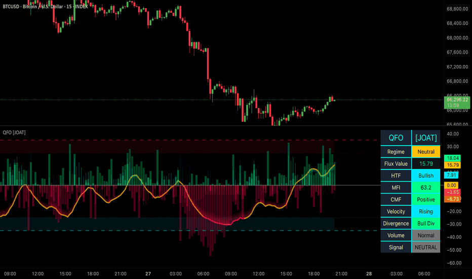
Smart Reversal EntrySmart Reversal Entry
Smart Reversal Entry is an open-source reversal-entry indicator built around one specific analytical idea:
after a short, directional three-candle expansion move, the first confirmed candle closing back in the opposite direction can create a structured reversal-entry opportunity when it appears in the correct EMA context.
This script is not designed to mark every bullish or bearish candle, and it is not intended to behave like a generic trend-following overlay, a standard candlestick-pattern indicator, or a broad “signal generator” that reacts to every small reversal. Its purpose is to measure short-term directional exhaustion in a standardized way, filter that move through an EMA context, require close-confirmed reversal behavior, and then project a fixed-risk trade structure directly on the chart for analysis and review.
The script also includes an internal background optimizer and review tables so users can compare how the same reversal framework behaves under different parameter combinations. These review tools are included to support study and comparison, not to imply future performance.
OPEN-SOURCE NOTE
This script is published open-source so users can inspect the logic directly, verify what the script is doing, and adapt parts of the workflow for their own research if they wish.
Even though the code is open, this description is intentionally detailed because many TradingView users do not read Pine Script. The goal is for a user to understand what the script does, how it works, why its parts belong together, and how it may be used in practice without having to study the code line by line.
OVERVIEW
At a high level, the script does six things:
1. It measures whether the last three candles produced a directional move large enough to matter in pip terms.
2. It checks whether price is positioned on the correct side of a selected EMA filter.
3. It requires the current candle to close in the opposite direction as confirmation of a possible reversal.
4. It maps a fixed stop-loss and a selectable take-profit multiple directly onto the chart.
5. It tracks projected trade outcomes and summarizes them in a review table and a daily PnL table.
6. It runs a hidden background optimizer over multiple EMA and move-threshold combinations so the user can compare the current settings to an internal parameter sweep.
The script is therefore meant to function as a complete reversal-entry and review framework rather than as a single-purpose candle-pattern marker.
CORE IDEA
Many reversal-style tools identify isolated candles or basic candlestick formations, but they do not standardize the market context around them.
This script is built around the idea that a reversal signal becomes more meaningful when three specific things happen together:
1. price has already made a clear short-term directional move,
2. that move is large enough to matter relative to the chosen pip structure,
3. and the next confirmed candle closes back in the opposite direction while price remains on the correct side of an EMA filter.
The model is intentionally narrow.
It does not try to identify every turning point in the market.
It does not try to classify broad market structure.
It does not use discretionary support and resistance interpretation.
It does not rely on vague candle descriptions such as “looks weak” or “looks exhausted”.
Instead, it defines reversal-entry conditions using a fixed sequence:
first measure a three-candle directional push,
then filter it using EMA context,
then require an opposite close-confirmed candle,
then project a standardized risk framework,
then review the resulting projected outcomes over time.
That narrower focus is the main reason this script exists in its current form.
WHY THIS SCRIPT IS NOT A SIMPLE MASHUP
This script combines multiple components, but they are not included simply to place more features into one publication.
Each component has a specific function inside the same analytical workflow:
- The EMA filter defines directional context.
- The three-candle move measurement defines whether a short-term push is large enough to qualify.
- The reversal candle confirmation defines the actual entry trigger.
- The pip-based stop-loss and RR framework standardize trade projection.
- The summary and daily review tables organize projected outcomes into a readable review structure.
- The internal optimizer compares the same reversal logic across multiple hidden EMA and move-threshold combinations.
These layers are interdependent.
Without the three-candle move measurement, the script would react to many small candles that do not represent meaningful short-term expansion.
Without the EMA filter, the script would lose its directional context and become a more generic reversal marker.
Without the close-confirmed reversal candle, the script would identify momentum but not the actual reversal-entry moment.
Without the risk projection layer, the user would still need to manually draw the entry, stop, and target after every signal.
Without the review tables, the user would have less organized feedback when reviewing results under the selected settings.
Without the internal optimizer, the user would see only the current configuration and not how the same logic behaves across a broader parameter range.
For that reason, the script is intended as a single reversal-entry framework, not as a random collection of unrelated features.
WHAT THE SCRIPT DOES
The script identifies reversal-entry setups using a strict, rule-based structure.
Long setup requirements:
- price must be above the selected EMA,
- the prior three candles must all be bearish,
- the combined bearish move across that sequence must reach the minimum pip threshold,
- the current candle must close bullish.
Short setup requirements:
- price must be below the selected EMA,
- the prior three candles must all be bullish,
- the combined bullish move across that sequence must reach the minimum pip threshold,
- the current candle must close bearish.
When a valid signal appears, the script can:
- place a BUY or SELL label,
- project a fixed stop loss in pips,
- project a take-profit level using the selected RR multiple,
- draw TP/SL boxes,
- draw an entry line,
- keep historical projected trades visible for later review,
- summarize projected outcomes in a summary table,
- summarize recent daily projected behavior in a daily PnL table.
The script also evaluates an internal optimizer in the background. That optimizer tests multiple EMA lengths and minimum-move combinations using the same reversal logic and displays the best-performing parameter combination inside the summary table over the shared analysis window.
HOW THE SCRIPT WORKS
1) EMA CONTEXT FILTER
The script uses a single EMA as a directional filter.
For long setups:
price must close above the selected EMA.
For short setups:
price must close below the selected EMA.
This does not turn the script into a pure trend-following system. Instead, it acts as a directional context filter so that reversal entries are only considered when price is positioned on the chosen side of the EMA.
In practical terms, the EMA filter is used to reduce context-free reversal signals. A bullish candle appearing after a bearish push is not enough by itself. The script still wants price to be trading above the selected EMA for longs, and below it for shorts.
2) THREE-CANDLE DIRECTIONAL MOVE MEASUREMENT
The script looks at the three candles immediately before the signal candle.
For a long setup:
those three candles must all be bearish.
For a short setup:
those three candles must all be bullish.
The script then measures the total directional move across that sequence in pip terms.
For long setups, it calculates the bearish move from the open of the first candle in the sequence to the close of the third bearish candle.
For short setups, it calculates the bullish move from the open of the first candle in the sequence to the close of the third bullish candle.
That move must be at least as large as the user-defined “Minimum 3-Candle Move (Pips)” setting.
This is one of the key parts of the script’s logic. It ensures that the setup is not based on three arbitrary candles, but on a directional push that is large enough to meet the minimum threshold selected by the user.
3) REVERSAL CANDLE CONFIRMATION
After the three-candle directional push is identified, the current candle must close in the opposite direction.
For long setups:
the current candle must close bullish.
For short setups:
the current candle must close bearish.
This requirement is intentionally strict. The script does not treat intrabar movement or unfinished candles as a valid signal. Signals are confirmed only when the bar closes.
This matters because a reversal that looks valid intrabar can disappear by the close. By waiting for close confirmation, the script reduces premature signal marking.
4) COOLDOWN FILTER
The script includes a cooldown period between signals.
Once a signal has fired, a new signal is not allowed until a defined number of bars has passed. In the current implementation, that cooldown is handled internally.
The purpose of this filter is to reduce signal clustering and prevent the chart from producing multiple nearby entries from the same short-term market behavior.
5) PIP-BASED RISK PROJECTION
When a valid signal appears, the script creates a projected trade framework using:
- entry at the signal close,
- a fixed stop-loss distance in pips,
- a take-profit level based on the selected risk/reward multiple.
This makes the projection logic standardized across signals.
For long setups:
- stop loss is placed below entry,
- take profit is placed above entry.
For short setups:
- stop loss is placed above entry,
- take profit is placed below entry.
The script can draw:
- entry line,
- TP box,
- SL box,
- BUY / SELL label,
- TP / SL hit labels.
This projection layer is not meant to claim that a setup will succeed. Its purpose is to reduce manual chart annotation and make the behavior of the signal model easier to inspect after the fact.
6) SAME-BAR TP/SL PRIORITY RULE
The script uses a strict and conservative rule when both target and stop would appear to be touched on the same bar after entry:
if TP and SL are both reached on the same bar, SL takes priority.
This is an important implementation detail because it directly affects projected statistics. It makes the review logic more conservative and avoids optimistic ambiguity when bar data alone cannot determine exact intrabar order.
7) SHARED ANALYSIS WINDOW
The script uses a shared analysis window internally.
Projected results and optimizer comparisons are evaluated over a rolling historical range rather than over the full unlimited chart history. This keeps the internal review process more controlled and makes the optimizer comparison consistent inside the same defined lookback window.
8) INTERNAL OPTIMIZER
One of the script’s more advanced components is the internal optimizer.
The optimizer runs in the background and is intentionally not exposed as a user-facing optimization panel. Instead of asking the user to manually test every variation, the script internally evaluates combinations of:
- 10 EMA values,
- 10 minimum-move thresholds.
That produces 100 total internal combinations.
Each combination uses the same reversal logic:
- EMA context,
- three-candle directional sequence,
- minimum move threshold,
- opposite close-confirmed candle,
- same stop-loss and RR structure.
The optimizer then tracks projected wins, losses, net R, gross profit, and gross loss for each combination, and the summary table displays the current best combination based on the script’s internal comparison rules.
This optimizer is not intended to present a “perfect setting”. It is a comparative review aid that helps the user understand how the same reversal framework behaves across multiple hidden parameter combinations.
WHAT MAKES THIS SCRIPT ORIGINAL
This script uses familiar technical-analysis building blocks such as:
- EMA filtering,
- candle-sequence logic,
- pip-based move measurement,
- fixed stop-loss projection,
- risk/reward mapping,
- performance review tables.
Those building blocks are not original by themselves.
The originality of this script is not in inventing a completely new primitive indicator. The originality lies in how these familiar elements are arranged into one tightly defined reversal-entry workflow:
EMA context
→ three-candle directional expansion
→ minimum pip-threshold validation
→ opposite candle close confirmation
→ fixed-risk trade projection
→ on-chart review
→ internal background parameter comparison
That full sequence is the main reason this script exists as its own publication.
It is not intended to be simply another EMA filter, another candlestick marker, another TP/SL visualizer, or another optimizer dashboard. It is specifically a short-term reversal-entry framework that combines directional context, expansion measurement, confirmation logic, risk mapping, and review in one workflow.
WHAT APPEARS ON THE CHART
Depending on settings, the chart may display:
- EMA line,
- BUY labels,
- SELL labels,
- signal-bar background highlights,
- entry line,
- TP box,
- SL box,
- TP hit labels,
- SL hit labels,
- summary table,
- daily PnL table.
Users who want a cleaner chart can disable some visual layers and keep only the ones most relevant to their workflow.
HOW TO USE THE SCRIPT
A practical workflow is:
1. Add the script to a standard candlestick chart.
2. Select the EMA length you want to use as directional context.
3. Set the minimum three-candle move threshold in pips.
4. Set the pip preset correctly for the instrument, or use manual pip size if needed.
5. Choose the stop-loss distance in pips.
6. Select the RR mode used for take-profit projection.
7. Wait for a valid long or short setup to appear.
8. Use the projected entry, stop, and target structure as a chart-analysis framework rather than as a blind instruction.
9. Review projected trade behavior in the summary table and daily table.
10. Compare your selected settings with the optimizer’s best internal combination, but do not treat the optimizer output as a guaranteed best future configuration.
This script is best understood as a structured decision-support and reversal-review tool, not as a self-sufficient trading system.
SETTINGS REFERENCE
Signal Settings
- EMA Length: sets the EMA used as the directional filter.
- Minimum 3-Candle Move (Pips): defines how large the directional three-candle move must be before a reversal candle can qualify.
Pip Settings
- Pip Preset: selects a predefined pip-size interpretation for common instrument types.
- Manual Pip Size: allows direct control when the selected symbol needs a custom pip conversion.
Risk Management
- Stop Loss (Pips): sets the fixed stop-loss distance in pip units.
- Take Profit RR: sets the projected target multiple relative to the stop-loss distance.
Visual Settings
- Show Buy/Sell Labels: shows or hides the signal labels.
- Highlight Signal Bars: adds background color to signal bars.
- Show Entry Line: shows or hides the projected entry line.
- Show TP/SL Hit Labels: controls whether projected outcomes are labeled.
- Show TP Hit Labels: controls TP hit labels specifically.
- Show SL Hit Labels: controls SL hit labels specifically.
Summary Table
- Show Summary Table: enables or disables the main review table.
- Table Position: sets the table location.
- Table Text Size: controls summary-table text size.
Daily PnL Table
- Show Daily PnL Table: enables or disables the daily review table.
- Daily Table Position: sets the daily table location.
- Daily Table Text Size: controls daily-table text size.
INTERNAL LOGIC NOTES
The current code also includes internal settings that are not exposed as user-facing optimization controls. These include:
- signal cooldown,
- shared analysis window,
- maximum stored closed-trade visuals,
- hidden optimizer activation,
- internal optimizer parameter combinations.
These internal elements exist to keep the public interface simpler while still allowing the script to maintain consistent review behavior in the background.
IMPORTANT PRACTICAL NOTE ON PIP SIZE
The script uses pip-based calculations for:
- the minimum three-candle move,
- stop-loss distance,
- take-profit distance,
- optimizer comparison logic.
Because of that, correct pip interpretation is extremely important.
If signals appear too frequent, too rare, too compressed, or visually inconsistent for the instrument being analyzed, the first setting to verify is Pip Preset or Manual Pip Size.
This matters especially for:
- gold symbols,
- 5-digit forex symbols,
- JPY forex pairs,
- indices and CFD-style instruments,
- custom broker symbols with unusual decimal formatting.
LIMITATIONS AND SHORTCOMINGS
This script has important limitations:
- It is a short-term reversal model, not a full market-structure engine.
- It only evaluates one specific reversal pattern based on a three-candle directional push and an opposite close-confirmed candle.
- It does not use support/resistance structure, volume profile, or discretionary context.
- It relies on pip conversion, so poor pip settings can distort signal behavior.
- The internal optimizer compares parameter combinations only inside the defined shared analysis window.
- The optimizer output is a comparative review tool, not a guarantee that the best historical combination will remain best in future market conditions.
- Projected results depend on the script’s own simplified outcome logic.
- If TP and SL are both touched on the same bar, SL is prioritized by design, which makes the logic more conservative but also affects outcome statistics.
- Historical projected trades and review metrics are chart-based review aids, not proof of tradable real-world execution.
- No reversal-entry model can remove all false signals or all regime-dependent behavior.
For those reasons, the script should be used as a structured analysis and review framework, not as a promise of future profitability.
WHO THIS SCRIPT MAY BE USEFUL FOR
This script may be useful for traders who:
- want a rules-based short-term reversal-entry model,
- want EMA-based directional context,
- want a minimum expansion threshold before a reversal is allowed,
- want fixed-risk trade projection on the chart,
- want review tables for projected outcomes,
- want background comparison of multiple EMA and move-threshold combinations.
It may be less suitable for traders who:
- want a broad trend-following system,
- want a discretionary support/resistance engine,
- want a multi-pattern candlestick library,
- want a fully automated strategy with no outside confirmation,
- want outcome metrics interpreted as live performance promises.
DISCLAIMER
This script is provided for educational and informational purposes only.
It does not constitute financial, investment, or trading advice.
Market conditions change, historical behavior does not guarantee future results, and users should perform their own analysis, validation, and risk management before using the script in live decision-making. インジケーター