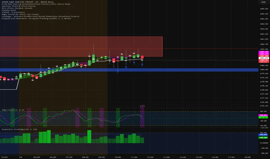
Quantum Momentum Wave [Pineify]Quantum Momentum Wave
Quantum Momentum Wave is a signed peak-momentum oscillator paired with a Kaufman-style adaptive filter. Instead of measuring the net change from one point to another, the wave scans the full lookback window and returns the largest absolute price displacement with its original sign. The wave is linearly smoothed and then tracked by an adaptive signal line, so entry markers fire on context-filtered reversals rather than every momentum flip.
Key Features
Signed peak-momentum engine that isolates the strongest move inside the lookback
Linear regression smoothing to tame the step-change behavior of raw peak readings
Adaptive signal line that speeds up when the wave is stretched and slows down in noise
Zone-filtered BUY and SELL markers that only fire when the wave is past zero in the opposite direction
Gradient fill between the wave and zero — bullish above, bearish below
Alerts for reversal setups and for zero-line regime shifts
How It Works
The core function is a QMW scan. On each bar it walks the last Momentum Lookback bars, computes price minus each historical bar, and keeps the comparison that produced the largest absolute change. It returns that value with its original sign. So a -6 reading means the single strongest move inside the window was a 6-unit drop, even if the bar-to-bar change right now is small.
Raw peak readings step when a new candle takes over as the dominant move, so the output is passed through linear regression over the Signal Smoothing length. LR fits a straight line through the recent raw values and returns its endpoint, preserving signed direction while cutting short-term jitter.
The adaptive signal runs a Kaufman-style update on top of the smoothed wave. Its coefficient is the ratio of the wave's absolute value to the sum of its recent absolute one-bar changes. When momentum is clearly extended and directional, the ratio is high and the signal follows quickly. When the wave oscillates near zero, the ratio collapses and the line nearly freezes.
How the Components Work Together
Three layers combine into one output. The peak scan answers how hard has price moved inside the window, not just where it ended. Linear regression answers what is the underlying direction of the peak reading after filtering out one-bar swaps between competing peak bars. The adaptive signal answers when has that direction actually shifted by providing a responsive reference line.
Entries layer a location filter on top. A crossover only qualifies when the wave is on the opposite side of zero — buys look for the wave turning up while stretched below zero, sells for the wave rolling over while stretched above it. Crosses near the midline are ignored because they tend to be low-conviction flips without prior displacement, so the setup is biased toward reversals from extended states rather than trend-chasing entries.
Trading Ideas and Insights
BUY triangles below zero can flag exhaustion of a downside push and a possible rotation back toward the mean
SELL triangles above zero can flag fading upside strength after an extended rally
Zero-line crosses act as broader regime markers; alerts on those can frame intraday bias
During strong trends the wave may stay on one side of zero for many bars. Counter-trend BUY or SELL labels in that state often need extra confirmation from price structure or higher-timeframe context
Signals are context aids, not standalone trade instructions. Past reactions at these conditions do not guarantee future ones.
Unique Aspects
The momentum calculation returns the peak signed displacement within the lookback, not a simple close-minus-close value. The reading stays elevated while the dominant move is still inside the window, which tracks the strongest displacement in memory rather than just endpoint delta
The adaptive signal uses a non-standard variation of Kaufman's efficiency ratio — absolute wave value divided by total absolute wave travel — tuned for oscillator input rather than raw price
Entry markers require both a crossover and a zone match. No label prints for a crossover that happens in the neutral zone around zero, which filters out the weakest setups
How to Use
Add the indicator to the chart and start with the defaults. The thicker line is the Quantum Wave; the fainter line is the Adaptive Signal
Read the wave color and the gradient fill to see which side of zero the wave is on and how stretched it is
Watch for BUY triangles when the wave is clearly below zero and turning up through the signal line
Watch for SELL triangles when the wave is clearly above zero and turning down through the signal line
Configure alerts for buy, sell, or zero-cross conditions if you want notifications outside the chart
Customization
Source Data (default: close) — Price series used for the peak momentum scan
Momentum Lookback (default: 14) — Window size for the peak displacement scan. Higher values capture broader swings; lower values react faster
Signal Smoothing (default: 9) — Linear regression length applied to the raw wave. Higher values produce a cleaner line with more lag
Bullish Color / Bearish Color — Wave color in positive and negative territory, and the BUY/SELL marker colors
Adaptive Signal Color — Color of the adaptive reference line; a subtle contrast against the wave usually reads cleanest
Limitations
Linear regression smoothing introduces a small amount of lag. On fast reversals the wave can reach the crossover a few bars after price has already moved
Because the adaptive ratio uses the wave's own value, very small wave readings near zero make the signal line nearly freeze. This is deliberate but means the reference reacts slowly while momentum is mild
Mean-reversion style BUY and SELL labels can occur repeatedly during strong trends. Pair them with price structure or higher-timeframe bias instead of using them in isolation
Conclusion
Quantum Momentum Wave is for traders who want an oscillator that reflects the strongest recent move rather than the endpoint delta. Its value comes from the combination of peak-momentum measurement, linear regression smoothing, and an adaptive reference line that only produces labels when the wave is both stretched past zero and visibly turning back. インジケーター

Artemis Volatility Bands PRO🟦 Artemis Volatility Bands PRO is a price-overlay volatility indicator built on the KernelLens Nadaraya–Watson regression library (a_jabbaroff/KernelLens/1). A single kernel estimate — selectable from eight classical kernel families — anchors the Basis line. Around it, two outer bands fan outward by a fixed multiple of the residual standard deviation, creating an envelope whose width is model-consistent with the kernel. The interior is washed with a 6-layer neon halo that mirrors the statistical density of price residuals under normality. A signal engine detects basis-breaks with confirming slope direction, guarded by Confirmed (zero-repaint) or Realtime mode. Twelve cohesive color themes, a theme-aware Dark / Light dashboard, and four opt-in alert conditions complete the indicator.
🟦 HOW IT WORKS
Artemis Volatility Bands PRO fuses two mathematical operations on every bar — a single kernel regression pass and a residual standard deviation calculation:
basis = kl.estimate(type, src, ℓ, α, period, phase, filter)
sigma = kl.confidenceBand(src, basis, window)
upper = basis + k · σ
lower = basis − k · σ
where ℓ is the Primary Bandwidth, k is the Band Multiplier, and window is the Residual σ Window. The kernel regression produces the Basis line, and the residual standard deviation (σ of price − basis) produces the per-σ band half-width.
This architecture collapses classical Bollinger band duality: in Bollinger bands, the moving average and volatility estimate live in different statistical universes. In Artemis, both emerge from a single kernel pass, so the envelope is internally consistent by construction. The Basis is always non-parametric, and the band width always measures deviation relative to the Basis, never to a disconnected moving average.
The library handles all weighted-sum computation, kernel weight evaluation, NA-safe iteration, division-by-zero guards, and input validation internally. Artemis Volatility Bands PRO does not reimplement any kernel math — every bug fix or optimization in the library automatically propagates to this indicator.
🟦 KERNEL LIBRARY INTEGRATION
Artemis Volatility Bands PRO imports the published KernelLens library and uses the following exports:
| Library Export | Used For |
|---|---|
| `kl.estimate()` | Unified dispatcher — routes to the correct kernel based on the user's Kernel Type dropdown. Called once per bar to produce the Basis line. |
| `kl.confidenceBand()` | Rolling residual standard deviation — computes σ of (source − basis) over the specified window. |
| `kl.trendState()` | Ternary trend detector — returns +1 (rising), 0 (flat), or −1 (falling) based on a 1-bar finite difference of the Basis. |
Every regression computation — kernel weight evaluation, NA-safe summation, bandwidth-aware loop termination — is delegated to the library. The indicator itself contains zero kernel math; it only orchestrates three library calls and aggregates their outputs into the band envelope and signal logic.
🟦 KERNEL REGRESSION & RESIDUAL VOLATILITY
**The Basis line** — A non-parametric kernel regression anchored to the user's choice of price source (default: close; also supports hl2, ohlc4, custom). Eight kernel families available:
| Kernel | Behavior | Best For |
|---|---|---|
| Rational Quadratic | Multi-scale mixer; α controls stretch | Default, balanced responsiveness |
| Gaussian / RBF | Canonical smoother, infinitely differentiable | Smooth trend, minimize noise |
| Periodic | Resonates with a known repetition distance p | Cyclic markets, seasonal patterns |
| Locally Periodic | Periodic × gaussian blend | Seasonal + trend drift |
| Epanechnikov | MSE-optimal, compact support | Minimal tail contamination |
| Tricube | LOWESS standard, near-Gaussian profile | Fast computation, robust |
| Triangular | Simplest compact kernel | Lightweight, real-time responsiveness |
| Cosine | Raised-cosine, smooth boundary transition | Smooth rolloff, professional appearance |
Three filter modes applied on top of the raw kernel estimate:
| Filter | Description | Use Case |
|---|---|---|
| No Filter | Single-pass Nadaraya–Watson | Rawest output, maximum responsiveness |
| Smooth | Double-pass: kernel applied to its own output | Cleaner, slightly more lag |
| Zero Lag | Ehlers de-lagging: 2·raw − smooth | Sharpens edges without increasing lag |
**Residual volatility** — Once the Basis is computed, the per-bar residual is (source − basis). The residual standard deviation is the rolling σ of this residual over a configurable window (default: 14 bars). This is the model-consistent volatility estimate — price deviations are measured relative to the kernel Basis, guaranteeing alignment between trend and volatility.
**Band levels** — upper = basis + k · σ and lower = basis − k · σ, where k is the Band Multiplier (default: 2.0, Bollinger-style). The multiplier is user-adjustable from 0.5 (tight) to 5.0 (wide).
🟦 SIGNAL ENGINE
Artemis fires Long / Short signals when price breaks the Basis with a confirming slope direction:
Long → close > basis AND basis rising
Short → close < basis AND basis falling
The signal state is persistent — once a direction flips, it remains latched until the opposite condition fires. This state machine (vii ∈ {−1, 0, +1}) ensures the Basis hue stays coherent across bars even when the raw trigger is a single-bar event.
Signal markers fire ONLY on the bar the state flips, not on every bar that satisfies the raw condition. This keeps the chart uncluttered and mirrors how discretionary traders consume trend-flip information.
**Signal Mode** — Two gating options:
| Mode | Behavior | Repaint |
|---|---|---|
| Confirmed | Signals fire ONLY after the bar closes via `barstate.isconfirmed` | Zero repaint, fully reliable for live trading |
| Realtime | Signals fire on the current (open) bar as soon as the condition is met | Fastest reaction; signal may vanish if price reverses before bar closes |
Historical repainting never occurs at any Signal Mode value. The library's `_phase` parameter shifts every kernel center into the past by that many bars, so historical bars' plotted values are final once confirmed.
🟦 6-LAYER NEON HALO VISUALIZATION
The interior between the Basis and each outer band is filled with a 6-layer gradient: 5 interior step plots plus the outer band, creating a stepped transparency schedule that mirrors the statistical density of price residuals under normality.
**Transparency schedule:**
| Layer | Transparency | Meaning |
|---|---|---|
| Outer band ↔ 1st interior | 70 % | Densest layer |
| 1st ↔ 2nd | 78 % | |
| 2nd ↔ 3rd | 85 % | |
| 3rd ↔ 4th | 90 % | |
| 4th ↔ 5th | 95 % | |
| 5th ↔ Basis | 98 % | Nearly invisible fade to centerline |
Every transparency value is scaled by the Gradient Intensity input (0–100 %), so the user can dial the visual density from invisible (0) to heavy fills (100).
**Color assignment:**
- Upper band + gradient: Bearish theme hue (short signal color)
- Lower band + gradient: Bullish theme hue (long signal color)
- Basis line: Slope-adaptive color (thBull when rising, thBear when falling, previous color on flat bars)
**Signal markers** — Two-layer neon glow plotshapes:
- Halo: size.small, 40 % opaque theme hue (glow layer)
- Core: size.tiny, 100 % opaque theme hue (bright center)
🟦 THEME SYSTEM
Twelve cohesive color palettes tuned to every trading aesthetic. One selection drives every visual component — Basis line, outer bands, gradient halos, long / short signal markers, dashboard accents — all sharing the same bull / bear / neutral color axes:
| Theme | Bull | Bear | Usage |
|---|---|---|---|
| Tropic | Cyan steel | Deep orange | Default, electric contrast |
| Amber | Warm amber | Indigo blue | Fire tones |
| Pastel | Sky blue | Soft lavender | Cool arctic glow |
| Cyber | Neon lime | Hot crimson | Cyber terminal aesthetic |
| Helios | Bright gold | Scarlet | Solar warmth |
| Electric | Electric aqua | Magenta | High-voltage neon |
| Candy | Neon green | Hot pink | Dark energy pop |
| Bloomberg | Terminal orange | Cyan | Wall Street finance heritage (PRO) |
| Solar | Solarized olive | Crimson | Developer palette, easy on eyes (PRO) |
| Royal | Imperial gold | Deep purple | Luxury signature (PRO) |
| Midnight | Deep navy | Dark crimson | Dark depth |
| Graphite | Near-black | Silver grey | Monochrome minimal |
**Dashboard display modes** — Dark (black background, bright accents) or Light (white background, darker accents), auto-adapting visual contrast regardless of chart background.
🟦 DASHBOARD
A 2-column, 9-row theme-aware status panel that updates only on the last bar (zero historical overhead). Supports Dark and Light display modes, six docking positions, and four text sizes. Renders via `force_overlay = true` on the main price chart.
| Row | Label | Content |
|---|---|---|
| Header | ARTEMIS PRO | DARK / LIGHT |
| Theme | Theme | Active palette name |
| Divider | KERNEL | — |
| Type | Type | Selected kernel type |
| Bandwidth ℓ | Bandwidth ℓ | Primary bandwidth + Phase φ |
| Basis | Basis | Current Basis value in chart mintick format |
| Divider | VOLATILITY | — |
| Residual σ | Residual σ | Current residual standard deviation |
| Signal | Signal | ▲ LONG / ▼ SHORT / ━ FLAT (direction-colored) |
🟦 ALERT CONDITIONS
Four opt-in alert conditions, each gated by its own toggle:
| Alert | Fires When |
|---|---|
| Long Signal | Price breaks above the Basis with a rising slope (confirmed state flip) |
| Short Signal | Price breaks below the Basis with a falling slope (confirmed state flip) |
| Upper Band Touch | Price touches or exceeds the upper outer band (raw crossover) |
| Lower Band Touch | Price touches or falls below the lower outer band (raw crossunder) |
Band touch alerts are useful as pre-signal early warnings in trending markets. Signal alerts are gated by the Signal Mode setting, so Confirmed mode ensures zero-repaint alerts suitable for live trading.
All alerts use `alertcondition()` for maximum compatibility with TradingView's alert system including webhooks. Messages are structured as `"Artemis Volatility Bands: "` for easy parsing in downstream automation.
🟦 RECOMMENDED PRESETS
| Trading Style | Bandwidth ℓ | Filter | Residual σ Window | Phase |
|---|---|---|---|---|
| Scalper | 10–20 | No Filter | 8–10 | 1 |
| Day Trader | 20–40 | Smooth | 14 | 2 |
| Swing | 30–60 | Smooth | 20–40 | 2 |
| Position | 60–120 | Smooth | 40–60 | 3 |
**Bandwidth tuning** — Smaller ℓ produces a tighter fit to price and faster reaction; larger ℓ produces smoother curves and more stability. Experiment with ℓ in your preferred style's range, then adjust the Residual σ Window and Filter mode for visual smoothness.
**Phase tuning** — Phase = 0 is live (flickers on the current bar); Phase = 2 is the recommended balance; Phase = 3+ adds margin against noise at the cost of lag. Historical charts are immutable at any phase value.
🟦 KERNEL-ONLY DESIGN PHILOSOPHY
Artemis Volatility Bands PRO contains zero classical technical analysis bolt-ons. No Bollinger Bands, no Keltner Channels, no linear regression, no ATR, no moving averages — only kernel regression and residual volatility. This kernel-only architecture guarantees that:
1. **Internal consistency** — The Basis and band width emerge from a single statistical model, not from mixing independent techniques.
2. **Unified parameterization** — All visual outputs (Basis, bands, gradient) are controlled by a single set of kernel-theoretic parameters.
3. **No analytical compromise** — Every choice in the indicator is mathematically motivated; no ad-hoc decorations.
The philosophy is defensive: traders who layer Artemis on top of their own edge strategies get a pure kernel-regression envelope that will not conflict with classical-TA signals already in use. Traders seeking a standalone kernel-based indicator get a complete, coherent system.
🟦 COMPATIBILITY
- Pine Script v6
- All exchanges, all asset classes (crypto, forex, equities, commodities, indices)
- All timeframes (1 minute through Monthly)
- Both Dark and Light chart themes — visual elements auto-adapt to chart background
- No exchange-specific logic — fully deterministic
Indicator renders on the main overlay chart with `force_overlay = true`. No secondary panes, no subplot logic.
🟦 TECHNICAL NOTES
- **Library dependency** — `import a_jabbaroff/KernelLens/1` — all kernel regression math is delegated to the published library
- **Plot budget** — 2 outer bands + 10 gradient interior plots + 1 Basis + 1 transparent anchor + 4 signal shapes + 12 fills + 4 alertconditions = 34 outputs, well under Pine's 64-output hard limit (50 % margin)
- **Table** — Single `var table` created once on `barstate.islast` with `force_overlay = true`; dashboard renders on the main chart pane, zero historical overhead
- **No persistent drawing objects** — no `box.new`, `line.new`, no `array.new`; all visuals are plots and fills
- **Opacity convention** — every user-facing opacity / transparency input follows `0 = invisible, 100 = fully opaque`; conversion to Pine's native transparency is centralized in a single helper function (`f_opac`)
- **Non-repainting** — inherits from the library's `_phase` parameter; no `request.security`, no lookahead, no future-bar leakage at any phase value
- **Residual consistency** — The residual σ is computed as `ta.stdev(source − basis, window)`, ensuring the band width always measures deviation relative to the kernel Basis
🟦 DISCLAIMER
Artemis Volatility Bands PRO is a technical analysis indicator built on the KernelLens Nadaraya–Watson regression library. It is provided solely for educational and research purposes and does not constitute financial, investment, or trading advice.
Kernel regression is a local smoothing technique. It estimates the mean of a source series in the neighborhood of the current bar based on historical data, but it does not predict future prices, does not generate trading signals on its own, and does not guarantee the profitability of any strategy built on top of its output. The signal engine is a mechanical detector of basis breaks and slope direction — not a forecast — and should always be combined with broader context: higher-timeframe structure, volatility regime, liquidity, news, and risk management.
Past performance of any model does not guarantee future results. Markets contain systemic risks that cannot be eliminated by any amount of mathematical rigor. Responsibility for any trading decisions rests entirely with the user. Always apply sound capital management, conduct your own independent analysis, and never risk capital you are not prepared to lose.
The author assumes no liability for direct or indirect losses incurred through the use of Artemis Volatility Bands PRO or the underlying KernelLens library. インジケーター

インジケーター

インジケーター

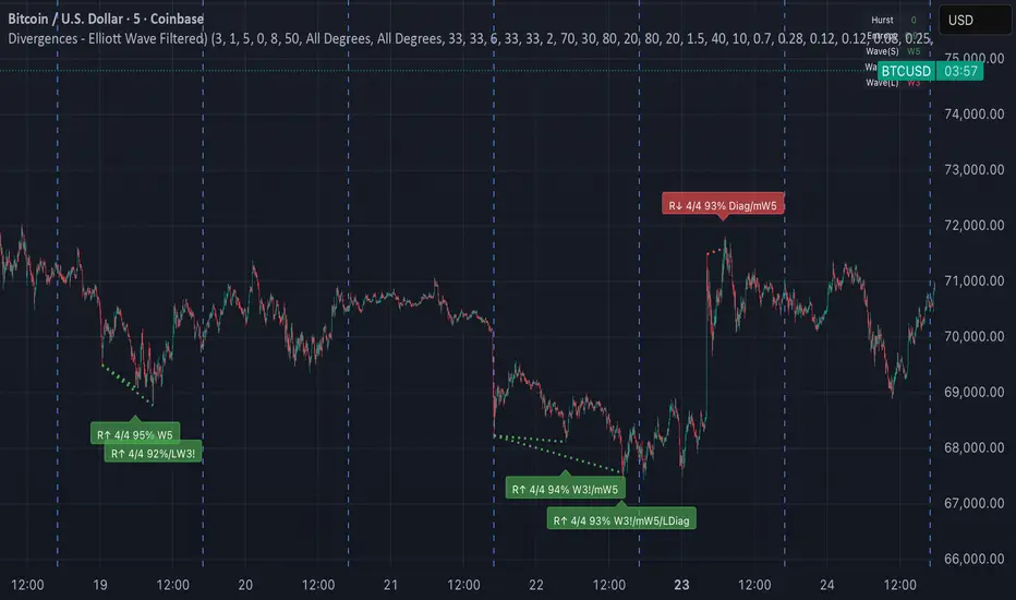
Divergences - Elliott Wave FilteredDivergences — Elliott Wave Filtered
A multi-oscillator divergence detection system that filters signals through a three-degree Elliott Wave engine and Bayesian probability fusion. Distinguishes between Regular divergences (reversal signals at wave ends) and Hidden divergences (continuation signals during corrections) using wave position scoring, Hurst regime analysis, and statistical quality metrics.
What It Does
This indicator scans for price-oscillator divergences across four technical indicators (RSI, Stochastic RSI, MFI, ROC) and validates them against real-time Elliott Wave structure. Unlike standard divergence indicators that fire indiscriminately, this system employs a wave-context gate — divergences only trigger if they align with specific wave positions (e.g., W5 endings for reversals, W2/W4 depths for continuations) across Small, Medium, and Large degrees.
Regular Divergences (Reversal): Price makes higher high / lower low while oscillator makes lower high / higher low. Filtered for W5, Diagonal, Corrective C, Triangle E, and W4/W2 endings where trend exhaustion is probable.
Hidden Divergences (Continuation): Price makes higher low / lower high while oscillator makes lower low / higher high. Filtered for W2, W4, and Corrective C positions where trend resumption is probable.
The Six Analytical Pillars
Multi-Oscillator Concordance : Requires minimum 2-of-4 oscillators (RSI, Stoch RSI, MFI, ROC) to simultaneously register divergence, eliminating single-indicator false positives.
Tri-Degree Wave Engine : Runs independent swing detection on Small (micro), Medium (minor), and Large (primary) degrees to determine if the divergence occurs at a significant wave node.
Wave Position Scoring : Assigns base probabilities (0.0–1.0) to wave positions — W5 (0.92), Diagonal (0.88), W2 (0.38), W4 (0.42), etc. — with separate score tables for Regular vs Hidden divergence contexts.
Cross-Degree Modifiers : Boosts probability when multiple degrees agree (e.g., Small=W5 + Medium=W5) or penalizes when they conflict (e.g., Small=W5 + Medium=W3).
Regime Detection : Integrates Hurst Exponent (mean-reversion vs persistence) and Shannon Entropy (market disorder) to weight divergence reliability — low Hurst (<0.5) favors reversal divergences, high entropy reduces signal confidence.
Bayesian Fusion : Combines concordance, z-score magnitude, wave context, trend agreement, and over-extension ratios through log-odds transformation to produce a final 0.0–1.0 probability score.
Key Features
Wave Type Filtering : Independent toggle sets for Regular vs Hidden divergences — e.g., allow W5+Diagonal+Triangle E for reversals, but only W2+W4+Corr C for continuations.
Slope Non-Intersection : Optional validation ensuring price does not cross the linear slope between P1 and P2 pivots (clean divergence requirement).
Dynamic Target Projection : Upon valid divergence, projects Fibonacci extension targets (61.8%, 100%, 161.8%) from the swing leg and plots invalidation levels (pivot ± ticks).
Degree Proximity Scaling : Small degree waves must be within 12 bars of divergence, Medium within 24 bars, Large within 48 bars — ensuring temporal relevance.
Quality Gradient : Impulse and Diagonal patterns receive quality scores (0.0–1.0) based on momentum, channel alignment, and alternation, scaling the base wave position probability.
Trend Agreement Check : Validates that divergence direction opposes (Regular) or aligns with (Hidden) the detected wave trend direction across degrees.
Inputs & Parameters
Divergence Detection
Pivot Left/Right Bars: Confirmation delay and lookback for pivot detection (default 3/1).
Min/Max Bars P1→P2: Time window constraints for valid divergence legs (default 5–unlimited).
Cooldown Bars: Minimum spacing between same-direction signals to prevent clustering (default 8).
Require Slope Non-Intersection: Toggle strict linear slope validation.
Wave Filter — Regular vs Hidden
Enable wave filter: Master toggle for each divergence type.
Degree to check: Any, Small, Medium, Large, or All Degrees (consensus requirement).
Allowed wave positions: Independent toggles for W5, Diagonal, W3, W2, W4, Corr C, Triangle E, and No Context.
Multi-Oscillator Concordance
Individual length settings for RSI (33), Stoch RSI (33, %K 6), MFI (33), ROC (33).
Min concordance: Required number of oscillators showing divergence (default 2 of 4).
OB/OS Zones: Overbought/oversold thresholds for RSI (70/30), Stoch (80/20), MFI (80/20).
Statistical Quality & Bayesian Weights
Z-score threshold: RSI deviation sensitivity (default 1.5).
Hurst lookback/entropy bins: Regime calculation windows.
Fusion weights: Concordance (0.28), Z-score (0.12), Hurst (0.12), Entropy (0.08), Wave context (0.25), Over-extension (0.08), Trend agreement (0.07).
Prior log-odds: Base bias adjustment (−3 to +3).
Min Score: Probability threshold for signal emission (default 0.85).
Wave Engine (Three Degrees)
Small: Left 3–30, Right 1–3, Min swing 0.08%.
Medium: Left 10–80, Right 1–5, Min swing 0.20%.
Large: Left 25–200, Right 2–10, Min swing 0.50%.
Wave-div proximity: 12 bars (Small), scaled 2×/4× for Medium/Large.
How to Read It
Divergence Labels:
R↑ (Green): Regular Bullish divergence — price lower low, oscillator higher low. Expect reversal up.
R↓ (Red): Regular Bearish divergence — price higher high, oscillator lower high. Expect reversal down.
H↑ (Teal): Hidden Bullish divergence — price higher low, oscillator lower low. Expect continuation up.
H↓ (Orange): Hidden Bearish divergence — price lower high, oscillator higher high. Expect continuation down.
Label Annotations: Format "Type Concordance/Total Score% WavePos" — e.g., "R↑ 3/4 92% W5/mW5" indicates 3 of 4 oscillators agree, 92% Bayesian probability, Small=W5, Medium=W5.
Dotted Lines: Connect P1 (previous pivot) to P2 (current pivot) showing the divergence slope.
Target Lines: Horizontal dashed lines at T1 (61.8%), T2 (100%), T3 (161.8%) projected from the divergence leg.
Invalidation Line: Solid grey line at the pivot price ± tick buffer — crossing this invalidates the divergence setup.
Dashboard (Top-Right): Displays current Hurst (green <0.5 mean-reverting, red >0.5 trending), Entropy (high = disorder), and detected wave positions for S/M/L degrees.
Signal Logic & Validation
Base Conditions: Price pivot confirmed, oscillator divergence detected, concordance ≥ minimum, within P1–P2 time window, cooldown satisfied.
Wave Filter Gate: Divergence bar must be within proximity window of a classified wave end (W5, Diag, W2, W4, etc.) on the specified degree(s).
Bayesian Calculation: Each component (concordance, z-score, Hurst, entropy, wave context, over-extension, trend) is converted to log-odds, weighted, summed with prior, and transformed back to probability.
Emission Threshold: Final probability must exceed Min Score (default 85%) to plot signal.
Over-Extension Ratio: Measures leg length vs previous similar leg — ratios >2.0 increase reversal probability (exhaustion signature).
Important Notes
Wave Position Scoring: Regular and Hidden divergences use inverted score tables. W5 scores 0.92 for Regular (strong reversal) but only 0.15 for Hidden (weak continuation). Conversely, W2 scores 0.38 for Regular but 0.90 for Hidden.
Cross-Degree Conflict: When degrees disagree (e.g., Small=W5 bullish, Medium=W3 bullish continuation), the system applies conflict penalties (−0.20 to −0.28) to the composite score, often suppressing the signal unless other factors compensate.
Hurst Interpretation: Hurst < 0.5 (mean-reversion regime) adds probability to Regular divergences (reversal expected) and reduces Hidden divergence scores. Hurst > 0.5 (trending) does the opposite.
Entropy Impact: High entropy (>0.7) indicates chaotic, non-cyclical market conditions — the system reduces confidence in all divergences during high entropy regimes.
Non-Intersection Validation: When enabled, the system checks that no intermediate bar crosses the linear interpolation between P1 and P2 pivots, ensuring "clean" divergence without whipsaw noise.
Quality Scaling: Impulse patterns are scored on momentum (W3 strength), channel parallelism, and alternation (W2 vs W4 slope difference). Higher quality waves boost the base position score by up to 30%.
No Repainting: Uses confirmed pivots (right bars ≥ 1) and historical bar indexing. Once a divergence is plotted at P2 confirmation bar, it remains fixed.
Mathematical Summary
Wave Position Base Scores (Regular)
W5 = 0.92, Diagonal = 0.88, Corr C = 0.65, Tri E = 0.60,
W4 = 0.42, W2 = 0.38, Neutral = 0.50, W3 = 0.12
Wave Position Base Scores (Hidden)
W2 = 0.90, W4 = 0.88, Corr C = 0.70, Neutral = 0.50,
W5 = 0.15, W3 = 0.35
Cross-Degree Modifiers
Triple Agreement = +0.20 (Tri Boost)
Dual Agreement = +0.15 (Agree Boost)
Single High vs Others Low = -0.20 to -0.28 (Conflict Penalty)
Bayesian Fusion
L = PriorLO + Σ(Weight_i × log(p_i / (1 - p_i)))
Posterior = 1 / (1 + exp(-L))
Impulse Quality
Quality = (Momentum × 0.35) + (Channel × 0.35) + (Alternation × 0.30)
FinalWaveScore = BaseScore + (BaseScore - 0.5) × Quality × 0.3
インジケーター

Artemis Regression Bands🟦 Artemis Regression Bands is a kernel-driven volatility envelope indicator built on the KernelLens Nadaraya–Watson regression library (a_jabbaroff/KernelLens/1). A single kernel estimate — selectable from eight classical kernel families — anchors the Fair Value line. Around it, three residual-standard-deviation bands (±1σ, ±2σ, ±3σ) fan outward with either Linear or Exponential spacing, producing a statistically grounded envelope far cleaner than the classical close-stdev approach used by legacy Bollinger-style indicators. A four-gate Romb signal engine overlays buy / sell diamond markers when price pokes through the outermost enabled σ boundary and reverses back inside.
🟦 HOW IT WORKS
Artemis calls the KernelLens library's unified dispatcher once per bar to build the Fair Value line, then queries three additional library exports to derive the band widths, slope direction, and residual σ:
```
fair = kl.estimate (type, src, ℓ, α, period, phase, filter)
sigma = kl.confidenceBand(src, fair, window)
slopeVal = kl.slope (fair, 1)
trendSt = kl.trendState (fair, 1)
dev = baseMult · sigma
upper1 = fair + 1·dev lower1 = fair − 1·dev
upper2 = fair + 2·dev lower2 = fair − 2·dev
upper3 = fair + k3·dev lower3 = fair − k3·dev (k3 = 3 Linear | 4 Exp)
```
The library handles all weighted-sum computation, loop-depth selection, NA-safe iteration, division-by-zero guards, and input validation internally. Artemis contains zero kernel math — every bug fix or optimization in the library automatically propagates to this indicator.
🟦 KERNEL LIBRARY INTEGRATION
Artemis imports the published KernelLens library and uses the following exports:
| Library Export | Used For |
|---|---|
| `kl.estimate()` | Unified dispatcher — routes to the correct kernel based on the user's Kernel Type dropdown. Called once per bar to produce the Fair Value line. |
| `kl.confidenceBand()` | Rolling standard deviation of the (source − Fair Value) residual. Drives the band half-widths on every bar. |
| `kl.slope()` | Discrete first derivative of the Fair Value line. Feeds trend flip alerts. |
| `kl.trendState()` | Ternary classifier (+1 rising / −1 falling / 0 flat) of the Fair Value line. Drives the slope-adaptive color, the kernel trend confluence filter, and the dashboard Trend row. |
Every regression computation — kernel weight evaluation, NA-safe summation, bandwidth-aware loop termination, residual stdev, finite-difference slope — is delegated to the library. The indicator itself only orchestrates the four library calls and layers the visual pipeline on top.
🟦 EIGHT KERNEL FAMILIES
A single Kernel Type dropdown selects any of the eight kernels shipped with the KernelLens library. Each is a different mathematical smoother with its own statistical character:
| Kernel | Formula | Best For |
|---|---|---|
| Rational Quadratic | (1 + d² / (2·α·ℓ²))^(−α) | Multi-scale mixer; α controls stretch. Recommended default. |
| Gaussian / RBF | exp(−d² / (2·ℓ²)) | Canonical smoother; infinitely differentiable. |
| Periodic | exp(−2·sin²(π·d/p) / ℓ²) | Resonates with a known repetition distance p. |
| Locally Periodic | Periodic × Gaussian | Seasonal patterns with slow trend drift. |
| Epanechnikov | (3/4)·(1 − u²), \|u\| ≤ 1 | MSE-optimal; compact support, no tail contamination. |
| Tricube | (70/81)·(1 − \|u\|³)³, \|u\| ≤ 1 | LOWESS standard; near-Gaussian compact profile. |
| Triangular | (1 − \|u\|), \|u\| ≤ 1 | Simplest compact kernel; cheapest to compute. |
| Cosine | (π/4)·cos(π·u/2), \|u\| ≤ 1 | Raised-cosine; smooth boundary transition. |
Because the dropdown feeds the library's `kl.estimate()` dispatcher directly, every kernel inherits the same three-mode filter layer (No Filter / Smooth / Zero Lag) and the same non-repainting guarantees — there is no special case per kernel in Artemis.
🟦 FILTER LAYER
A second dropdown applies an optional post-processing layer on top of the raw Nadaraya–Watson estimate:
| Filter | Formula | Trade-off |
|---|---|---|
| No Filter | ŷ = ŷ_raw | Single-pass kernel. Rawest output, most reactive. |
| Smooth | ŷ = K(ŷ_raw) | Double-pass — kernel applied to its own output. Cleaner line, slightly more lag. |
| Zero Lag | ŷ = 2·ŷ_raw − K(ŷ_raw) | Ehlers de-lagging identity — sharpens edges without adding lag. |
The filter is resolved entirely inside `kl.estimate()`, so switching modes incurs no runtime cost beyond the extra kernel pass.
🟦 RESIDUAL-σ BAND ENGINE
Artemis bands are statistically grounded on the residual standard deviation — not on raw close stdev as in classical Bollinger indicators. The residual is computed as:
```
residual = src − fair
sigma = ta.stdev(residual, window) // via kl.confidenceBand()
```
Because Fair Value is already an unbiased local estimate of the source, the residual is a zero-mean noise series and its stdev captures **only the portion of price variance that the kernel could not explain**. This produces three benefits over the classical approach:
1. **Tighter bands in trending regimes** — close-stdev widens during strong trends because the trend itself inflates the variance; residual-σ does not, because the kernel absorbs the trend.
2. **Faster reaction to volatility regime changes** — residual-σ tightens as soon as the kernel fits well, and widens the instant the market breaks out of the kernel's neighborhood.
3. **True statistical interpretation** — under the assumption of locally Gaussian residuals, ±1σ / ±2σ / ±3σ enclose approximately 68 % / 95 % / 99.7 % of near-term price variation. The traditional close-stdev envelope carries no such interpretation.
A dedicated Residual σ Window input controls the lookback; typical values range from 50 (reactive, scalping) to 300 (stable, position trading).
🟦 BAND SPACING MODES
Two spacing presets shape the outward fan of the three σ bands:
| Mode | Multipliers | Character |
|---|---|---|
| Linear | 1·, 2·, 3· | Classical Bollinger-style uniform steps. Predictable, symmetric. |
| Exponential | 1·, 2·, 4· | Fibonacci-flavored — outer band (4σ) is reserved for genuine blow-off excursions. |
Base Multiplier scales all three bands uniformly (default 1.0). The formula is:
```
band_level = fair ± (baseMult · k · sigma) k ∈ {1, 2, k3}
```
where k3 resolves to 3 in Linear mode and 4 in Exponential mode. Every band has an independent visibility toggle, so minimalist users can run ±1σ only, swing traders ±3σ only, or any combination.
🟦 FOUR-GATE ROMB SIGNAL ENGINE
The Romb engine prints buy / sell diamond markers when price pokes through the outermost enabled σ band and reverses back inside. Four sequential gates protect against false entries:
| Gate | Logic | Purpose |
|---|---|---|
| 1 — Crossover | `ta.crossunder(high, triggerUp)` / `ta.crossover(low, triggerDn)` | Detects the reversal back through the outer band. |
| 2 — Warm-up | Residual σ computable for N consecutive bars | Blocks signals during the early kernel-settlement window. |
| 3 — Confluence | Fair Value slope aligns with the reversal direction | Optional PRO filter — Sell Romb requires falling kernel, Buy Romb requires rising kernel. |
| 4 — Cooldown | Minimum bar gap since the last same-side Romb | Prevents signal clustering on a single extended poke-and-reverse sequence. |
A Signal Mode toggle layers on top:
- **Confirmed** — signals fire only on `barstate.isconfirmed`; zero repaint on closed bars.
- **Realtime** — signals fire live on the current open bar; faster reaction, may vanish if price reverses before close.
Each confirmed signal is rendered as a two-layer neon diamond:
- **Halo** — `size.small`, 40 % transparent theme hue (glow layer).
- **Core** — `size.tiny`, fully opaque theme hue (bright center).
The halo renders first so the core sits cleanly on top, producing a sharp luminous marker that reads instantly even on dense price charts.
🟦 ADAPTIVE OUTER-BAND TRIGGER
The Romb engine does not hard-code the ±3σ band as the signal trigger. Instead, it resolves the outermost currently-enabled band on every bar:
```
triggerUp = show3 ? upper3 : show2 ? upper2 : show1 ? upper1 : na
triggerDn = show3 ? lower3 : show2 ? lower2 : show1 ? lower1 : na
```
The result is an envelope that respects the user's visibility choices:
| Visible Bands | Romb Fires At |
|---|---|
| ±1σ + ±2σ + ±3σ | ±3σ (default) |
| ±1σ + ±2σ | ±2σ |
| ±1σ only | ±1σ |
| All off | no signals |
Diamond positioning follows the same trigger, so the glyph always floats ~0.3σ outside whatever envelope is actually drawn on the chart. The behavior matches user intent: the band I can see is the band that fires signals.
🟦 NON-REPAINTING BEHAVIOR
Artemis inherits non-repainting behavior directly from the KernelLens library's `_phase` parameter. A single Phase input (default 2) shifts the kernel center into the past by that many bars:
- **Phase = 0** — live estimate, flickers on the current bar (real-time only; history is immutable).
- **Phase = 1** — 1-bar lag, non-repainting once the bar is confirmed.
- **Phase = 2** — recommended balance between freshness and stability (default).
- **Phase = 3+** — extra margin against erratic ticks, higher lag.
Historical repainting never occurs at any phase value. The library contains no `request.security` calls, no lookahead, and no array rotation that could leak future data. Every historical bar's plotted Fair Value, band, and Romb signal is final once confirmed.
🟦 VISUAL PIPELINE
**σ Band Outlines** — Three upper bands (±1σ / ±2σ / ±3σ) in progressively lighter `thBear` hues, three lower bands in progressively lighter `thBull` hues. Hidden bands collapse to na via their individual visibility toggles; the outline widths share a single Band Line Width input.
**Tapered Gradient Fills** — Six fills drawn between the Fair Value line and each σ band. Opacity scales progressively from ±1σ (densest, most opaque) to ±3σ (lightest, most transparent), creating a halo that mirrors the statistical density of price residuals under normality. Master Fill Opacity input (0 = invisible, 100 = fully opaque) scales all three fills uniformly.
**Fair Value Line** — Slope-adaptive color resolver swaps between `thBull` (rising kernel) and `thBear` (falling kernel). Flat bars retain the previous color so the line never flashes neutral on a perfectly horizontal tick. Width is user-controlled (1–5 px).
**Romb Diamonds** — Two-layer neon glow at the adaptive trigger band; halo + core rendering described above.
**Bar Coloring** — Optional theme-aware candle coloring driven by the Fair Value slope. Off by default; when enabled it paints every bar with the active theme's bull / bear hue based on the current trend state.
🟦 THEME SYSTEM
Twelve cohesive color palettes drive every visual component — Fair Value line, σ band outlines, gradient fills, Romb diamonds, bar coloring, and dashboard accents — all sharing the same four color axes (`thBull`, `thBear`, `thNeutral`, `thSignal`):
| Theme | Bull | Bear |
|---|---|---|
| Tropic | Cyan steel | Deep orange |
| Amber | Warm amber | Indigo blue |
| Pastel | Sky blue | Soft lavender |
| Cyber | Neon lime | Hot crimson |
| Helios | Bright gold | Scarlet |
| Electric | Electric aqua | Magenta |
| Candy | Neon green | Hot pink |
| Bloomberg | Terminal orange | Cyan |
| Solar | Solarized olive | Crimson |
| Royal | Imperial gold | Deep purple |
| Midnight | Deep navy | Dark crimson |
| Graphite | Near-black | Silver grey |
A separate Display Mode toggle (Dark / Light) controls the dashboard palette independently of the chart theme — so a Bloomberg chart theme with a Light dashboard is a valid configuration, as is Midnight chart + Dark dashboard.
🟦 DASHBOARD
A 2-column, 12-row theme-aware status panel that updates only on the last bar (zero historical overhead). Supports Dark and Light display modes, six docking positions, and four text sizes. Renders via `force_overlay = true` on the main price chart.
| Row | Label | Content |
|---|---|---|
| Header | ARTEMIS | DARK / LIGHT |
| Theme | Theme | Active palette name |
| Kernel | Kernel | Selected kernel type |
| Divider | REGRESSION | — |
| Bandwidth | Bandwidth ℓ | Bandwidth value / Phase offset φ |
| Filter | Filter | No Filter / Smooth / Zero Lag |
| Fair Value | Fair Value | Current Fair Value in chart mintick format |
| Divider | BANDS | — |
| Spacing | Spacing | Linear 1·/2·/3· or Exp 1·/2·/4· |
| Residual σ | Band σ | Rolling residual standard deviation |
| Trend | Trend | ▲ BULL / ▼ BEAR / ━ FLAT (bull/bear colored) |
| Last Romb | Last Romb | ▲ BUY (N ago) / ▼ SELL (N ago) — bull/bear colored |
**Zebra-stripe layout** — alternating `dashBg` / `dashBgAlt` row backgrounds improve scan-ability on narrow cells. Section dividers (REGRESSION, BANDS) use a third background tone (`dashSection`) with the theme's bull accent as the header color — preserving brand identity across both Display Modes.
🟦 ALERT CONDITIONS
Six opt-in alert conditions, each gated by its own toggle:
| Alert | Fires When |
|---|---|
| Bullish Trend Flip | Fair Value slope crosses from ≤ 0 into positive territory |
| Bearish Trend Flip | Fair Value slope crosses from ≥ 0 into negative territory |
| Buy Romb | Confirmed Buy Romb fires — all four signal gates passing |
| Sell Romb | Confirmed Sell Romb fires — all four signal gates passing |
| Upper Band Touch | Price touches or exceeds the outermost enabled upper band |
| Lower Band Touch | Price touches or falls below the outermost enabled lower band |
All alerts use `alertcondition()` for maximum compatibility with TradingView's alert system including webhooks. Messages are structured as `"Artemis Regression Bands: "` for easy parsing in downstream automation. Touch alerts are off by default (can be noisy in trending markets); the four core alerts are on by default.
🟦 RECOMMENDED PRESETS
| Style | Bandwidth ℓ | Filter | Phase | Spacing | σ Window | Chart |
|---|---|---|---|---|---|---|
| Scalper | 10–20 | No Filter | 1 | Linear | 50–80 | 1m–5m |
| Day Trader | 20–40 | Smooth | 2 | Linear | 80–120 | 15m–1h |
| Swing | 30–60 | Smooth | 2 | Linear or Exp | 100–200 | 4h–1D |
| Position | 60–120 | Smooth or Zero Lag | 3 | Exp | 200–300 | 1D–1W |
**Kernel type tuning**
- **Trending instruments** — Rational Quadratic (α = 1–3) or Gaussian. Smooth multi-scale response.
- **Mean-reverting instruments** — Epanechnikov or Tricube. Compact support keeps the band envelope tight.
- **Session-cyclic patterns** — Periodic (with p = session length in bars) or Locally Periodic. Resonates with known cycles.
**Romb filter tuning** — Keep Kernel Trend Confluence ON for high-conviction setups only. Switch OFF on range-bound instruments to capture both sides of the oscillation.
🟦 COMPATIBILITY
- Pine Script v6
- All exchanges, all asset classes (crypto, forex, equities, commodities, indices)
- All timeframes (1 minute through Monthly)
- Both Dark and Light chart themes — the Display Mode toggle controls dashboard palette independently
- No exchange-specific logic — fully deterministic
🟦 TECHNICAL NOTES
- **Library dependency** — `import a_jabbaroff/KernelLens/1` — all kernel regression, residual σ, slope, and trend-state math is delegated to the published library.
- **Plot budget** — 6 band plots + 1 Fair Value anchor + 1 Fair Value visible + 6 gradient fills + 4 Romb plotshapes + 1 barcolor = well under Pine's plot limits.
- **Table** — Single `var table` rebuilt on `barstate.islast` with `force_overlay = true`; zero historical overhead.
- **Signal state** — Two `var int` cooldown anchors (`lastSellBar`, `lastBuyBar`) seeded at −10000 so the very first bar always passes the gap test. A `var int stabCount` warm-up counter blocks signals during early kernel settlement.
- **No persistent drawing objects** — no `box.new`, `line.new`, no array rotations; every visual is either a plot or a single-bar plotshape.
- **Adaptive trigger resolver** — Romb crossover detection, touch alerts, and diamond positioning all read from the same `triggerUp` / `triggerDn` resolver, so band visibility toggles stay semantically coherent across every layer of the indicator.
- **Non-repainting** — inherits from the library's `_phase` parameter; no `request.security`, no lookahead, no future-bar leakage at any phase value.
🟦 DISCLAIMER
Artemis Regression Bands is a technical analysis indicator built on the KernelLens Nadaraya–Watson regression library. It is provided solely for educational and research purposes and does not constitute financial, investment, or trading advice.
Kernel regression is a local smoothing technique. It estimates the mean of a source series in the neighborhood of the current bar based on historical data, but it does not predict future prices, does not generate trading signals on its own, and does not guarantee the profitability of any strategy built on top of its output. The residual-σ envelope describes past dispersion around the kernel estimate — not a forecast of future range — and should always be combined with broader context: higher-timeframe structure, volatility regime, liquidity, news, and risk management.
Past performance of any model does not guarantee future results. Markets contain systemic risks that cannot be eliminated by any amount of mathematical rigor. Responsibility for any trading decisions rests entirely with the user. Always apply sound capital management, conduct your own independent analysis, and never risk capital you are not prepared to lose.
The author assumes no liability for direct or indirect losses incurred through the use of Artemis Regression Bands or the underlying KernelLens library. インジケーター

Quant Edge Ribbon PRO🟦 Quant Edge Ribbon PRO is a multi-kernel divergence ribbon indicator built on the KernelLens Nadaraya–Watson regression library (a_jabbaroff/KernelLens/1). A primary kernel and eleven longer-bandwidth kernels form a dual-ribbon visualization driven by kernel regression mathematics, an integer trend score in , a theme-aware rendering pipeline, four user-configurable reference levels, and a PRO dashboard. All twelve kernels route through the unified library dispatcher, so the user may select any of the eight kernel families and any of the three filter modes from a single configuration panel.
🟦 HOW IT WORKS
Quant Edge Ribbon PRO calls the KernelLens library's unified dispatcher (`kl.estimate`) twelve times per bar — once for the primary kernel and once for each of the eleven outer kernels:
```
primary = kl.estimate(type, src, ℓ, α, period, phase, filter)
long00 = kl.estimate(type, src, ℓ + 1·s, α, period, phase, filter)
long01 = kl.estimate(type, src, ℓ + 2·s, α, period, phase, filter)
...
long10 = kl.estimate(type, src, ℓ + 11·s, α, period, phase, filter)
```
where ℓ is the Primary Bandwidth and s is the Bandwidth Step. All twelve kernels share the same kernel type, filter, shape α, period, and phase — only the bandwidth differs. This guarantees the ribbon behaves as a coherent spectrum of kernel scales rather than a mixture of unrelated signals.
The library handles all weighted-sum computation, loop-depth selection, NA-safe iteration, division-by-zero guards, and input validation internally. Quant Edge Ribbon PRO does not reimplement any kernel math — every bug fix or optimization in the library automatically propagates to this indicator.
🟦 KERNEL LIBRARY INTEGRATION
Quant Edge Ribbon PRO imports the published KernelLens library and uses the following export:
| Library Export | Used For |
|---|---|
| `kl.estimate()` | Unified dispatcher — routes to the correct kernel based on the user's Kernel Type dropdown. Called twelve times per bar, once for the primary kernel and once for each of the eleven outer kernels. |
Every regression computation — kernel weight evaluation, NA-safe summation, bandwidth-aware loop termination — is delegated to the library. The indicator itself contains zero kernel math; it only orchestrates twelve library calls and aggregates their outputs into the trend score.
🟦 THE TWELVE-KERNEL RIBBON ARCHITECTURE
**Primary kernel (the shortest, the anchor)** — A single kernel at bandwidth ℓ that serves two roles: (1) it is the reference baseline for the trend score calculation, and (2) it is plotted as a dedicated highlighted anchor line when the "Highlight Primary Kernel" toggle is ON.
**Eleven outer kernels (progressively wider)** — Kernels at bandwidths ℓ+1·s, ℓ+2·s, …, ℓ+11·s, where s is the Bandwidth Step (default: 1). Each outer kernel is plotted as a line on the main chart, all eleven sharing a single score-driven gradient color — so the entire outer ribbon shifts between the theme's bull and bear hues as the trend score moves between −11 and +11.
**Eleven inner ribbon plots (lagged primary snapshots)** — The primary kernel plotted at eleven time-lag offsets (0, 1, 2, …, 10 bars). The resulting visual is a gently flowing shadow that makes expansion and contraction of the outer ribbon easier to perceive. Opacity is user-controlled (default: 40 %).
🟦 INTEGER TREND SCORE
The trend score is a signed integer in , computed on every bar by eleven pairwise comparisons between the primary kernel (at progressive lag offsets) and the eleven outer kernels:
```
score = 0
for i in 0..10:
if primary < long_i:
score += 1
else:
score -= 1
```
**Semantic interpretation** — Each comparison pairs an older snapshot of the shortest kernel against a current snapshot of a progressively wider kernel. In an uptrend, past primary values are lower while current wider-kernel values have caught up above them — the inequality resolves positive on most pairs and the score climbs toward +11. The symmetric argument drives the score toward −11 in a downtrend.
**Score parity** — Because the score is a sum of eleven ±1 terms (score = 2k − 11, k ∈ ), it is always odd. Reachable values: { −11, −9, −7, −5, −3, −1, 1, 3, 5, 7, 9, 11 }. The score is never exactly zero.
🟦 STRENGTH CATEGORIZATION
The absolute score is bucketed into four bands, each with a matched label glyph used throughout the dashboard and the last-bar signal label:
| Score Range | Strength | Label |
|---|---|---|
| \|score\| = 1 | NEUTRAL | ▰▱▱▱ NEUTRAL |
| \|score\| ∈ {3, 5} | WEAK | ▰▰▱▱ WEAK BULL / WEAK BEAR |
| \|score\| = 7 | STRONG | ▰▰▰▱ STRONG BULL / STRONG BEAR |
| \|score\| ∈ {9, 11} | TRIPLE | ▰▰▰▰ TRIPLE BULL / TRIPLE BEAR |
The bull / bear suffix is driven by the sign of the score. The progress-bar glyphs (▰▱) give an instant at-a-glance read of confluence intensity without needing to parse the numeric value.
🟦 NON-REPAINTING BEHAVIOR
Quant Edge Ribbon PRO inherits non-repainting behavior directly from the KernelLens library's `_phase` parameter. A single Phase input (default: 2) shifts every one of the twelve kernel centers into the past by that many bars.
- Phase = 0 — live estimate, flickers on the current bar (real-time only; history is immutable)
- Phase = 1 — 1-bar lag, non-repainting once the bar is confirmed
- Phase = 2 — recommended balance between freshness and stability (default)
- Phase = 3+ — extra margin against erratic ticks, higher lag
Historical repainting never occurs at any phase value. The library contains no `request.security` calls, no lookahead, and no array rotation that could leak future data. Every historical bar's plotted value is final once confirmed.
🟦 VISUAL PIPELINE
**Outer Ribbon Gradient** — All eleven outer kernels are plotted with a single shared color driven by the trend score via `color.from_gradient(score, -11, 11, thBear, thBull)`. As the score walks across its range, the entire ribbon shifts continuously between the active theme's bearish and bullish hues — producing a smooth visual feedback loop between the math and the palette.
**Inner Ribbon Shadow Trail** — Eleven lag-shifted primary snapshots (primary through primary ) drawn in the theme's accent hue with user-controlled opacity. On a trending chart the trail visually expands; on a reversing chart it contracts. Adjust opacity from 0 (invisible) to 100 (fully opaque) — default 40 balances presence and subtlety.
**Primary Kernel Anchor Line** — The primary kernel plotted as a dedicated bold line in the theme's accent color at 80 % opacity, distinct from the shadow trail. Provides a clear centerline amid the ribbon flow. Toggleable.
**Oscillator Subplot** — The smoothed trend score plotted in a dedicated subplot with a score-gradient vertical fill between the score line and the zero line. Opacity is user-controlled. An optional bold score line (up to 4 px wide) overlays the fill for sharp numeric reading.
**Last-Bar Trend Label** — A right-anchored label at the current bar in the oscillator pane. Format: `▲ TRIPLE BULL 11 / 11` (bull) or `▼ WEAK BEAR −3 / 11` (bear). The label is deleted and redrawn on every bar, so only one instance is ever present on the chart.
🟦 OSCILLATOR STYLES
The oscillator subplot ships with two visual presets, selectable from the Oscillator Style dropdown:
| Style | Plot Style | Fill | Best For |
|---|---|---|---|
| Classic Gradient | `plot.style_line` (smooth curve) | Continuous vertical gradient from score to zero | Trend flow, slope momentum |
| Stepline | `plot.style_stepline` (staircase) | Stepped gradient mirroring the discrete score plateaus | Signal / threshold trading, discrete level crossings |
**Classic Gradient** produces a smooth curve traced through the smoothed score values, with the gradient fill flowing continuously between the score line and the zero line. This is the default and suits traders who read trend direction through slope and curvature.
**Stepline** renders each bar as a horizontal plateau joined to the next bar by a vertical edge. Because the raw score is always an odd integer in { −11, −9, …, 9, 11 }, the staircase visualization honors the score's true discrete nature — making it easier to identify exact threshold crossings (e.g. the moment the score enters the ±9 extreme zone). The fill inherits the same stepline style, so the entire oscillator pane stays geometrically consistent.
Both styles share the same opacity controls, score line toggle, and line width setting — only the geometry of the score line and its fill changes between them.
🟦 THEME SYSTEM
Ten cohesive color palettes tuned to the Quant Edge Ribbon PRO optical brand. One selection drives every visual component — outer ribbon gradient, inner ribbon accent, oscillator fill, reference lines, signal label, dashboard accents — all sharing the same bull / bear / accent color axes:
| Theme | Bull | Bear |
|---|---|---|
| Prism | Forest green | Crimson red |
| Focus | Cyan steel | Deep orange |
| Solar | Warm amber | Indigo red |
| Frost | Sky blue | Soft lavender |
| Laser | Neon lime | Hot crimson |
| Aurora | Bright gold | Scarlet |
| Plasma | Electric aqua | Magenta |
| Bloom | Mint green | Hot pink |
| Eclipse | Deep navy | Dark crimson |
| Carbon | Near-black | Silver grey |
The oscillator's zero line uses Pine's `chart.fg_color` so it auto-adapts to the actual chart background (white on dark charts, black on light charts) — independent of the Dashboard's Display Mode setting.
🟦 REFERENCE LEVELS
Four user-configurable horizontal reference lines mark the score's structural thresholds inside the oscillator subplot:
| Level | Style | Meaning |
|---|---|---|
| +11 / −11 | Dotted | Ceiling / floor — the mathematical maximum (every comparison aligned) |
| +9 / −9 | Dashed | Extreme zone — nine or more of the eleven comparisons agree on direction |
Each pair (±11 and ±9) has an independent opacity input (0–100 %). A master toggle (Show Reference Levels) collapses all four lines to fully transparent in a single branch — useful for minimalist layouts. An additional `showOsc` gate hides them automatically when the oscillator itself is disabled.
🟦 PRO DASHBOARD
A 2-column, 12-row theme-aware status panel that updates only on the last bar (zero historical overhead). Supports Dark and Light display modes, six docking positions, and four text sizes. Renders via `force_overlay = true` on the main price chart.
| Row | Label | Content |
|---|---|---|
| Header | Q-EDGE PRO | DARK / LIGHT |
| Theme | Theme | Active palette name |
| Kernel | Kernel | Selected kernel type |
| Divider | RIBBON | — |
| Primary ℓ | Primary ℓ | Primary bandwidth value |
| Span | Span | ℓ → ℓ + 11·s |
| Filter | Filter | No Filter / Smooth / Zero Lag |
| Divider | SCORE | — |
| Score | Score | ▲/▼ + integer score + " / 11" (bull/bear colored) |
| Bull / Bear | Bull / Bear | Bull comparison count / bear comparison count |
| Strength | Strength | ▰-bar + NEUTRAL / WEAK / STRONG / TRIPLE label |
| Primary | Primary | Primary kernel value in chart mintick format |
**Bull / Bear breakdown** — The eleven pairwise comparisons split into bulls (resolved +1) and bears (resolved −1). Always sums to 11, so this row gives a direct visual of how many kernel scales agree with the net direction.
🟦 ALERT CONDITIONS
Six opt-in alert conditions, each gated by its own toggle:
| Alert | Fires When |
|---|---|
| Bullish Flip | Score crosses from ≤ 0 into positive territory |
| Bearish Flip | Score crosses from ≥ 0 into negative territory |
| Extreme Bullish | Score reaches +9 or higher (first entry into the zone) |
| Extreme Bearish | Score reaches −9 or lower (first entry into the zone) |
| Full Confluence Up | Score hits +11 — every outer kernel aligned bullishly |
| Full Confluence Down | Score hits −11 — every outer kernel aligned bearishly |
All alerts use `alertcondition()` for maximum compatibility with TradingView's alert system including webhooks. Messages are structured as `"Quant Edge Ribbon PRO: "` for easy parsing in downstream automation.
🟦 RECOMMENDED PRESETS
| Style | Primary ℓ | Bandwidth Step s | Phase | Filter | Chart |
|---|---|---|---|---|---|
| Scalper | 8–16 | 1 | 1 | No Filter | 1m–5m |
| Day Trader | 16–32 | 1–2 | 2 | Smooth | 15m–1h |
| Swing | 25–50 | 1–2 | 2 | Smooth | 4h–1D |
| Position | 50–120 | 2–3 | 3 | Smooth | 1D–1W |
**Bandwidth Step tuning** — Step = 1 produces a tight ribbon where adjacent outer kernels sit visually close together. Steps of 2–4 spread the eleven outer kernels across a broader spectrum of scales, making expansion / contraction easier to read at a glance. Step 5–6 is reserved for very wide ribbons where each line represents a distinctly different time scale.
🟦 COMPATIBILITY
- Pine Script v6
- All exchanges, all asset classes (crypto, forex, equities, commodities, indices)
- All timeframes (1 minute through Monthly)
- Both Dark and Light chart themes — visual elements auto-adapt via `chart.fg_color`
- No exchange-specific logic — fully deterministic
🟦 TECHNICAL NOTES
- **Library dependency** — `import a_jabbaroff/KernelLens/1` — all kernel regression math is delegated to the published library
- **Plot budget** — 11 outer + 11 inner + 1 primary + 2 oscillator plots + 1 fill + 4 hlines = well under Pine's 64-plot limit
- **Table** — Single `var table` created once on `barstate.islast` with `force_overlay = true`; dashboard renders on the main chart pane, zero historical overhead
- **No persistent drawing objects** — no `box.new`, `line.new`, no `array.new`; the single trend label is deleted and recreated every bar so only one instance is ever present
- **Opacity convention** — every user-facing opacity input follows `0 = invisible, 100 = fully opaque`; conversion to Pine's native transparency is centralized in a single helper function (`f_opac`)
- **Non-repainting** — inherits from the library's `_phase` parameter; no `request.security`, no lookahead, no future-bar leakage at any phase value
- **Chart background adaptive** — the oscillator's zero line uses `chart.fg_color`, so it always renders with high contrast regardless of the user's chart color scheme
🟦 DISCLAIMER
Quant Edge Ribbon PRO is a technical analysis indicator built on the KernelLens Nadaraya–Watson regression library. It is provided solely for educational and research purposes and does not constitute financial, investment, or trading advice.
Kernel regression is a local smoothing technique. It estimates the mean of a source series in the neighborhood of the current bar based on historical data, but it does not predict future prices, does not generate trading signals on its own, and does not guarantee the profitability of any strategy built on top of its output. The integer trend score is a geometric summary of kernel alignments — not a forecast — and should always be combined with broader context: higher-timeframe structure, volatility regime, liquidity, news, and risk management.
Past performance of any model does not guarantee future results. Markets contain systemic risks that cannot be eliminated by any amount of mathematical rigor. Responsibility for any trading decisions rests entirely with the user. Always apply sound capital management, conduct your own independent analysis, and never risk capital you are not prepared to lose.
The author assumes no liability for direct or indirect losses incurred through the use of Quant Edge Ribbon PRO or the underlying KernelLens library. インジケーター

インジケーター
Delta Pressure Gauge [JOAT]Delta Pressure Gauge
Introduction
Delta Pressure Gauge is a pane-based oscillator that constructs a volume-weighted directional wave from bar-by-bar delta estimation, normalized using a rolling maximum to ensure consistent scaling across all instruments and timeframes. The oscillator measures the pressure imbalance between buying volume and selling volume, smoothed into a wave that reveals accumulation and distribution phases with high visual clarity. The indicator includes a money flow pressure line, a cumulative windowed delta cloud, divergence detection, and crossover signal dots.
Traditional volume indicators — OBV, CMF, MFI — measure volume flows using raw or price-weighted calculations that are difficult to compare across instruments or timeframes because their absolute values depend on the asset's volume profile. Delta Pressure Gauge normalizes everything to a -1 to +1 scale using a rolling maximum, producing readings that are immediately interpretable regardless of whether the asset trades 100 shares or 100 million. The wave design provides a visual rhythm that makes accumulation and distribution phases recognizable at a glance.
Core Concepts
1. Body-Quality Weighted Bar Delta
Each bar contributes a delta value based on direction (bullish = +volume, bearish = -volume) multiplied by the bar's body quality ratio (body size divided by total range). A full-body bar contributes 100% of its volume to delta. A doji bar with no body contributes 0%. This filtering reduces the noise contribution of indecision bars that add volume without directional information.
body_qual = math.abs(close - open) / math.max(high - low, syminfo.mintick)
bar_delta = bar_dir * volume * body_qual
2. Rolling Maximum Normalization
The raw wave EMA is normalized by dividing by the rolling maximum absolute value over the normalization window. Unlike percentile-based normalization, rolling maximum works reliably from the first bar, requires no minimum warmup period, and produces values that are always within the -1 to +1 range:
norm_ref = ta.highest(math.abs(raw_wave), i_norm)
wt1 = raw_wave / math.max(nz(norm_ref, 1.0), 1.0)
3. Windowed Cumulative Delta
Rather than using an all-time cumulative delta (which grows without bound and becomes dominated by early bars), the cumulative component uses a 30-bar rolling sum. This produces a medium-term delta bias that reflects the recent directional commitment of volume participants.
4. Money Flow Pressure Line
A separate money flow calculation weights volume by the ratio of price movement to range: (close - open) / range × volume. This captures the efficiency of price movement relative to its volume cost — high-momentum bars have larger weights than range-bound bars.
5. Divergence Detection
Bullish divergence is detected when the delta wave makes a higher low while price makes a lower low. Bearish divergence is the mirror. Detection uses confirmed pivot points on the wave with persistent previous-pivot storage, avoiding any ta.valuewhen type compatibility issues. Divergence lines are rendered directly on the oscillator pane.
Features
Wave Oscillator: Gradient area fill between wave and zero, color-coded by direction and intensity
Signal Line: Smoothed signal with direction-colored rendering
Histogram: Four-state colored momentum bars showing wave-signal separation and its rate of change
Crossover Dots: Large circles with glow rings at every wave/signal crossover
Zero-Line Cross Dots: Small markers when wave crosses the zero line
Overbought/Oversold Extreme Dots: Markers at extreme readings
Divergence Triangles and Lines: Yellow markers and connecting lines when divergence is detected
Cumulative Delta Cloud: Area fill showing 30-bar rolling delta direction
Money Flow Line: Purple secondary line for cross-confirmation
Volume Surge Markers: Cross markers when volume exceeds 2x average
12-Row Dashboard: Pressure state, wave values, histogram, signals, cumulative delta, money flow, volume ratio, divergence state
Input Parameters
Wave Channel Length: Fast EMA for wave construction (default: 10)
Wave Average Length: Signal line smoothing period (default: 21)
Rolling Norm Window: Window for rolling maximum normalization (default: 100)
Overbought/Oversold levels: Four configurable threshold lines
Divergence pivot lookback settings
How to Use This Indicator
Crossover Dots as Momentum Shifts
When the wave crosses above the signal line (green dot), buying pressure is accelerating relative to the smoothed baseline. This confirms a momentum pickup. The opposite for bearish crosses. These signals are strongest when they occur near or below the oversold line.
Zero-Line Confirmation
The wave crossing zero from below indicates that aggregate buying pressure over the wave window has turned net positive. This is a regime confirmation, not an entry signal in isolation, but it supports bullish bias when aligned with price structure.
Divergence at Extremes
Divergence is most meaningful when the wave is at or near an overbought or oversold extreme. A bullish divergence from the oversold zone (yellow triangle pointing up) suggests the distribution of buying pressure is shifting despite continued price weakness.
Cumulative Delta Direction
The blue-purple cloud shows whether the 30-bar rolling delta is net positive or negative. When the wave crosses bullishly and the cumulative delta is also positive, both the momentum and the persistent pressure agree.
Limitations
This indicator uses close-open direction to estimate bar delta. True bid-ask volume data (available only through specialized data providers) would be more precise. On instruments with significant wick activity (doji bars), this estimation introduces noise
Normalization by rolling maximum means a single extreme bar sets the scale for the entire norm window. One unusually large volume bar will compress all surrounding readings
Divergence detection requires enough bars for pivot confirmation. The pivot right-side lookback introduces a lag in divergence signals
This indicator measures volume pressure proxies, not actual institutional activity. Large volume does not always reflect institutional intent
Originality Statement
The body-quality weighting applied before delta smoothing is a deliberate design choice that reduces doji noise in a way that raw-volume or typical-price approaches do not. The rolling maximum normalization (rather than percentile or z-score) was chosen specifically because it operates reliably from the first bar without a warmup cliff, making the indicator immediately usable on limited datasets. The combination of a wave oscillator, cumulative delta cloud, and money flow line on a single pane provides three independent perspectives on the same underlying volume pressure question.
Disclaimer
This indicator is for educational and informational purposes only. Volume pressure readings are estimates derived from OHLCV data. They do not represent actual order flow or institutional positioning. Past divergence patterns do not predict future price reactions. Always apply appropriate risk management.
-Made with passion by officialjackofalltrades
インジケーター

インジケーター
インジケーター

インジケーター

インジケーター

インジケーター

インジケーター

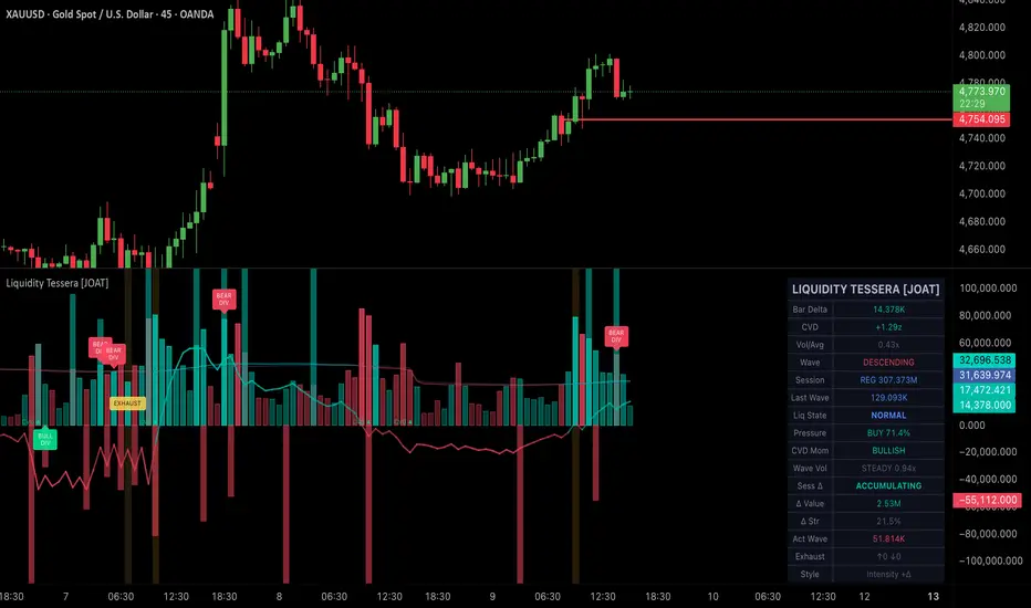
Liquidity Tessera [JOAT]Liquidity Tessera
Introduction
Liquidity Tessera is an advanced open-source volume intelligence pane that fuses Cumulative Volume Delta (CVD), Weis Wave volume clustering, multi-design intensity bars, volume absorption and climax detection, CVD momentum ribbon, liquidity exhaustion tracking, session-partitioned delta accumulation, and a comprehensive 16-row dashboard into a unified volume analysis system. This indicator transforms raw volume data into actionable intelligence about who controls the market — buyers or sellers — and whether that control is strengthening or weakening.
Standard volume indicators show you how much trading occurred. Liquidity Tessera shows you the character of that trading: whether volume is flowing in or out (CVD), whether volume waves are expanding or contracting (Weis Wave), whether institutions are absorbing supply or distributing into demand (absorption detection), and whether a move is reaching climactic exhaustion (climax and exhaustion signals). The indicator operates in its own pane below the price chart, providing a complete volume intelligence layer without cluttering price action.
Core Concepts
1. Cumulative Volume Delta (CVD)
CVD approximates the net buying and selling pressure by assigning each bar's volume as positive (buying) when the close is above the open, and negative (selling) when the close is below the open:
float barDelta = close > open ? volume : close < open ? -volume : 0.0
var float cvdRaw = 0.0
cvdRaw := nz(cvdRaw ) + barDelta
The cumulative sum of these deltas creates a running total of net order flow. Rising CVD indicates net buying pressure is accumulating; falling CVD indicates net selling pressure. The indicator offers optional normalization using a z-score approach (CVD relative to its rolling mean and standard deviation), which makes CVD comparable across different instruments and timeframes.
CVD divergences from price are particularly significant: when price makes a new high but CVD does not confirm (it stays below its recent high), it suggests the rally lacks genuine buying conviction and may be vulnerable to reversal.
2. Weis Wave Volume Clustering
The Weis Wave method groups volume into directional waves. Rather than looking at volume bar-by-bar, it accumulates volume during each directional swing. A wave reversal is triggered when price moves against the current wave direction by more than a configurable ATR-based threshold:
float waveThreshold = ta.atr(waveAtrLen) * waveAtrMul
// When price reverses by more than the threshold, the wave completes
// and accumulated volume is plotted as a single wave column
This reveals the Wyckoff-style volume pattern: are up-waves attracting more volume than down-waves (accumulation), or are down-waves attracting more volume (distribution)? The indicator tracks wave history and detects divergences between price swings and their corresponding wave volumes.
3. Volume Absorption Detection
Institutional absorption occurs when large players absorb selling pressure (or buying pressure) without allowing price to move significantly. The indicator detects this by identifying bars where volume is extremely high relative to average (above the configurable threshold, default 2x) but the price range is unusually small (below 50% of average range):
High volume + small range = someone is absorbing the opposite side's orders
This often occurs at the end of trends when institutions are building positions against the prevailing direction
Absorption bars are highlighted with a distinct amethyst color and labeled "ABS" on the chart.
4. Volume Climax Detection
A volume climax occurs when extreme volume (above the configurable threshold, default 3x average) coincides with a reversal candle pattern — specifically, a bar with a large wick-to-body ratio (wick > 2x body). This combination suggests that a massive influx of orders met strong opposition, creating a potential turning point. Climax bars are highlighted in fuchsia and labeled "CLIMAX."
5. Liquidity Exhaustion Tracking
The indicator tracks consecutive Weis Waves where volume declines from wave to wave. When two or more consecutive waves in the same direction show declining volume, it signals exhaustion — the trend is running out of fuel. This is a classic Wyckoff concept: a trend sustained by decreasing volume is unsustainable.
6. Delta Intensity Bar Coloring
Rather than simple up/down coloring, the indicator offers gradient-based bar coloring where the intensity of the color reflects the strength of the bar's delta relative to average volume:
float deltaStr = math.min(math.abs(barDelta) / volMA, 2.0) / 2.0
// Weak delta = faint color, strong delta = vivid color
baseCol := color.from_gradient(deltaStr, 0, 1,
color.new(TESS_INFLOW, 65), color.new(TESS_INFLOW, 0))
This means a green bar with faint color had weak buying conviction, while a vivid green bar had strong buying conviction — information not available from standard volume bars.
7. CVD Momentum Ribbon
A fast and slow EMA of the raw CVD create a momentum ribbon. When the fast CVD EMA is above the slow, delta momentum is bullish (buying pressure is accelerating). Crossovers between the two indicate shifts in delta momentum direction.
Features
Four Bar Design Modes: Solid (standard filled bars), Hollow (outline only), Intensity (transparency scales with volume relative to average), and Glass (semi-transparent with a stepline cap) — each providing a different visual emphasis
Weis Wave Histogram: Background columns showing completed wave volumes, colored by wave direction. Up-wave volumes plot above zero, down-wave volumes below
CVD Overlay: The cumulative delta line scaled to fit the volume pane, with gradient coloring from bearish (red) to bullish (teal) based on CVD value
Session Volume Accumulation: Separate tracking of pre-market, regular, and post-market session volumes and deltas, with session background coloring
Delta Pressure Score: A 0-100 percentage measuring net buying pressure over the last 20 bars. Above 60 = buy pressure dominant, below 40 = sell pressure dominant
Wave Volume Comparison: Real-time comparison of the current wave's volume against the previous wave, classified as Expanding, Steady, or Contracting
Liquidity State Classification: Categorizes the current bar as Absorption, Climax, Exhaustion, Spike, Dry-Up, or Normal based on the composite of all detection systems
Volume Spike Detection: Identifies bars where volume exceeds 2.5x average with a background highlight
Session Delta Bias: Tracks whether the current session's cumulative delta is net accumulating or distributing
16-Row Dashboard: Displays bar delta, CVD state, volume ratio, wave direction, session volumes, last wave volume, liquidity state, delta pressure, CVD momentum, wave volume comparison, session delta bias, delta strength, active wave volume, exhaustion counts, and bar style
Input Parameters
Cumulative Delta:
CVD Smoothing: EMA period for CVD smoothing (default: 14)
Normalize CVD: Toggle z-score normalization for cross-asset comparability (default: on)
CVD Ribbon Fast/Slow: EMA periods for the momentum ribbon (default: 8/21)
Wave Volume:
Wave ATR Multiplier: Threshold for wave reversal detection (default: 1.5)
Wave ATR Length: ATR period for wave threshold (default: 14)
Signals:
Absorption Vol Threshold: Volume multiple for absorption detection (default: 2.0)
Climax Vol Threshold: Volume multiple for climax detection (default: 3.0)
Toggles for wave divergence, absorption, climax, and exhaustion signals
Visuals:
Bar Style: Solid, Hollow, Intensity, or Glass (default: Intensity)
Toggles for delta intensity coloring, wave histogram, CVD overlay, CVD ribbon, session background, and dashboard
How to Use This Indicator
Step 1: Read the Liquidity State
Check the dashboard's Liquidity State. "Absorption" at support suggests institutions are buying. "Climax" after an extended move suggests a potential turning point. "Exhaustion" means the trend is losing volume fuel. "Normal" means standard conditions apply.
Step 2: Monitor CVD Direction
Rising CVD confirms uptrends; falling CVD confirms downtrends. CVD diverging from price is a warning sign. If price is making new highs but CVD is flat or declining, the rally may lack genuine buying support.
Step 3: Compare Wave Volumes
In a healthy uptrend, up-wave volumes should be larger than down-wave volumes. If down-wave volumes start exceeding up-wave volumes while price is still rising, distribution may be occurring. The Wave Volume Comparison metric in the dashboard tracks this automatically.
Step 4: Use Delta Pressure for Bias
The Delta Pressure score (0-100) provides a quick read on who controls the last 20 bars. Above 60 = buyers dominate. Below 40 = sellers dominate. Between 40-60 = balanced/contested.
Step 5: Watch for Signal Clusters
The most significant moments occur when multiple signals cluster: an absorption bar followed by a wave divergence during an exhaustion phase, for example, creates a high-conviction reversal setup. Single signals in isolation are less reliable.
Indicator Limitations
The CVD approximation (close > open = buying, close < open = selling) is a simplification. True order flow data requires Level 2/DOM data not available in Pine Script. This approximation works reasonably well on liquid instruments but is inherently imprecise
Volume data quality varies significantly across instruments and data providers. Forex "volume" is typically tick count, not actual traded volume. Crypto volume may include wash trading. The indicator's effectiveness depends on the quality of the underlying volume data
Weis Wave reversal detection depends on the ATR threshold parameter. Too small a threshold produces too many waves (noise); too large produces too few (missing genuine reversals). The optimal setting varies by instrument and timeframe
Absorption and climax detection use fixed ratio thresholds. What constitutes "extreme" volume varies across instruments and market conditions. The thresholds may need adjustment
Session volume tracking uses TradingView's built-in session detection, which may not align perfectly with all exchanges or instruments
The indicator operates in a separate pane and cannot overlay directly on price. Cross-referencing signals with price action requires visual comparison between panes
Originality Statement
This indicator is original in its comprehensive fusion of multiple volume analysis methodologies into a unified intelligence pane. While individual components (CVD, Weis Wave, volume absorption) exist separately, this indicator is justified because:
The integration of CVD, Weis Wave clustering, absorption detection, climax detection, and exhaustion tracking into a single system provides layered volume intelligence not available in any single existing indicator
The delta intensity bar coloring system uses gradient transparency based on delta strength, providing conviction information within the volume bars themselves
The liquidity state classification system synthesizes all detection subsystems into a single categorical assessment of current market conditions
Session-partitioned delta tracking reveals whether accumulation or distribution is occurring within specific market sessions
The CVD momentum ribbon provides a trend-following overlay on the delta data, identifying shifts in buying/selling momentum
Four distinct bar design modes (Solid, Hollow, Intensity, Glass) offer visual flexibility for different analysis preferences
Wave volume comparison with expanding/contracting classification automates Wyckoff-style wave analysis
Disclaimer
This indicator is provided for educational and informational purposes only. It is not financial advice or a recommendation to buy or sell any financial instrument. Trading involves substantial risk of loss. Volume analysis provides context about market participation but does not predict future price direction. Absorption, climax, and exhaustion signals are probabilistic patterns that can and do fail. CVD approximations are not equivalent to true order flow data. Always use proper risk management and conduct your own analysis. The author is not responsible for any losses incurred from using this indicator.
-Made with passion by officialjackofalltrades
インジケーター

RSI Divergence ProRSI Divergence Pro
Forget the classic RSI bouncing between 0 and 100 where you're left squinting at charts trying to spot divergences yourself.
RSI centers everything on zero — positive means bullish, negative means bearish, done. No mental math wondering if 45 is "almost oversold." Overbought/oversold zones adapt dynamically to the market instead of sitting frozen at 30/70.
Three divergence types detected automatically: Regular (trend reversal), Hidden (trend continuation), and — this is what nobody else has — Momentum Divergences: price is still climbing, but RSI is quietly losing steam. The warning signal before the classic divergence even becomes visible.
Armed State is the real killer feature: the indicator detects when a divergence is building but hasn't fired yet — green/red dots show you in real time "heads up, something's brewing." You see the trade before it exists.
Everything controlled by a single strength filter: one slider, zero clutter. High = fewer signals that hit. Low = see everything. Your call.
Arrows on chart, lines in the oscillator, info table, alerts — all built in, all toggleable. インジケーター

AG Pro Structure Labels [AGPro Series]AG Pro HH HL LH LL Structure Labels
Overview / What it does
AG Pro HH HL LH LL Structure Labels is a clean market-structure reader built to simplify price action without turning the chart into a wall of signals. Its core purpose is straightforward: identify confirmed swing highs and swing lows, classify them as HH, HL, LH, or LL, and connect those points in a visually readable structure path so traders can understand the current sequence of price development at a glance.
Many market structure tools try to do too much at once. They mix structure, signals, zones, pattern scoring, and trade suggestions into a single publication, which can make the chart heavier and the analytical purpose less clear. This script takes the opposite route. It focuses on one job only: making confirmed swing structure easier to read, follow, and interpret in real time as the chart evolves.
That design choice is what gives this script its value. Instead of asking the user to interpret disconnected highs and lows manually, the script builds a visible structure chain from confirmed pivots and labels each important step. The result is a chart that remains visually disciplined while still communicating trend continuation, structural weakening, and flow transitions in a simple and repeatable format.
This script is especially useful for traders who want structure clarity before they bring in any other layer of analysis. It can be used as a standalone structure map, or as a first-pass chart-cleaning tool before applying other concepts such as support and resistance, trend continuation logic, pullback analysis, breakout validation, or discretionary execution rules.
Unique Edge
The unique edge of this script is not that it attempts to predict where price will go next. Its strength is that it organizes confirmed structure in a way that is visually clean, logically consistent, and immediately usable on live charts.
Unlike many AG Pro scripts that are built around event detection, confluence scoring, price-zone visualization, setup quality filtering, or breakout logic, this publication is intentionally narrower and more focused. It is not a BOS/CHoCH event detector. It is not a liquidity-sweep model. It is not an order-block or fair-value-gap engine. It is not a breakout-quality, retest-quality, or pattern-quality scorer. It is also not a fixed reference-level tool such as a prior-day or prior-week high/low mapper. This script is a structure readability tool first and foremost.
That distinction matters.
Previous AG Pro releases often revolve around a specific trading event: a sweep, a break, a retest, a zone reaction, a continuation pattern, or a multi-factor confluence state. This script does not begin from an event. It begins from the swing chain itself. It asks a simpler question: what is the current sequence of confirmed highs and lows, and what does that sequence imply about market flow right now?
Because of that, the script fills a different role in the broader AG Pro library. It is closer to a structural map than a setup engine. It helps answer whether the chart is still printing constructive highs and lows, whether the sequence has started to weaken, or whether the structure is now leaning in the opposite direction. That makes it useful both on its own and as a foundation layer beneath other tools.
Another important differentiator is presentation discipline. The structure path provides continuity between pivots, while the label set communicates classification without unnecessary chart clutter. The compact floating HUD reinforces the current flow state without dominating screen space. Together, these choices make the script visually premium while keeping the chart readable.
Methodology
The script uses a confirmed pivot framework. Swing highs and swing lows are identified using left and right lookback parameters selected by the user. Because pivots require confirmation, labels appear only after the structure point is confirmed by the specified number of bars. This helps reduce noise and keeps the structure map grounded in confirmed rather than speculative swing points.
Once a new pivot high is confirmed, it is compared with the prior confirmed pivot high. If it exceeds the previous confirmed high, it is classified as HH. If it does not, it is classified as LH. The same logic applies on the low side: if a confirmed pivot low is above or equal to the previous confirmed pivot low, it is classified as HL; if it is lower, it is classified as LL.
The script also includes an ATR-based structure filter. This filter is designed to suppress micro-swings that are too small relative to current volatility, which helps maintain visual cleanliness on choppier charts. Instead of drawing every minor fluctuation, the script attempts to keep attention on swings that are more structurally meaningful for the selected sensitivity.
A structure path, shown as a clean zigzag line, connects the confirmed pivots that pass the filter. This gives the user an immediate visual map of the sequence rather than a collection of isolated labels. In practice, this is one of the most useful parts of the script because it turns the market’s swing progression into a readable path.
The floating HUD summarizes the current market-flow bias in a minimalist format. It is not intended to act as a trade signal. Its job is to provide a quick structural read so the user can see whether the recent chain is leaning bullish, bearish, or transitional according to the internal swing logic.
Signals & Alerts
This script is not designed as a one-click entry engine. Its alerts are structural, not predictive.
The publication includes alerts for newly confirmed HH, HL, LH, and LL prints, which can help users monitor structure development without staring at the chart continuously. It also includes alerts for structure-flow transitions when the internal trend state turns bullish or bearish.
These alerts are best understood as workflow alerts. They tell the user that structure has progressed into a new confirmed condition. They do not guarantee continuation, reversal, breakout success, or trade profitability. Their purpose is to improve awareness of structural change, not to replace independent analysis.
Key Inputs
Pivot sensitivity is controlled through left and right lookback values. Higher values usually produce fewer but more mature structure points, while lower values usually produce a faster and denser structure map.
The ATR filter can be enabled to reduce insignificant swings. This can be particularly helpful on lower timeframes or during periods of uneven, noisy price movement.
Users can also control whether the structure path is drawn and can adjust the visual typography for labels and HUD elements. These inputs allow the script to stay visually flexible across different chart styles and screen densities.
How this script differs from other AG Pro scripts
This distinction is central to the publication.
Many AG Pro scripts are built to evaluate the quality of a setup. They may score breakouts, retests, continuation patterns, reversal candles, pressure conditions, or confluence states. Others are built around zones and reactions, such as supply-demand mapping, premium-discount logic, fair value gaps, order blocks, or support-resistance behavior. Others focus on structural events such as BOS/CHoCH changes, liquidity sweeps, inducement traps, or session-specific reactions.
This script does none of those things.
It does not measure the quality of a signal.
It does not score a setup.
It does not project targets.
It does not identify fixed daily or weekly reference levels.
It does not try to map every institutional concept on the chart.
It does not attempt to be an all-in-one decision engine.
Instead, it provides a cleaner foundation: confirmed HH, HL, LH, and LL sequencing with a filtered structural path and a compact market-flow summary.
That is precisely why it is different from the previous AG Pro script as well. If the previous release was anchored to fixed price levels, event detection, or context-specific reactions, this script is anchored to swing continuity. If another AG Pro script answers where price reacted, where a sweep occurred, whether a breakout was strong, or whether a setup deserves a quality score, this one answers a more basic but highly important question: what is the confirmed structure chain doing right now?
In that sense, this script is less about trading events and more about structural readability.
Limitations & Transparency
This script uses confirmed pivots, which means it is not attempting to label unconfirmed structure in advance. As a result, there is an intentional delay equal to the confirmation logic chosen by the user. That delay is not a flaw; it is part of the design tradeoff required to avoid premature structure labels.
Like any pivot-based structure tool, output will vary depending on sensitivity settings, timeframe, market volatility, and symbol behavior. A lower sensitivity may reveal more swing detail but can also make the map denser. A higher sensitivity may create a cleaner structure path but may respond more slowly to local shifts.
The ATR filter is a visual-cleanliness tool, not a universal truth engine. It can help reduce noise, but different traders may prefer different levels of structural compression depending on how aggressively or conservatively they define meaningful swings.
This script should also not be interpreted as a complete trading plan. It does not include position sizing, stop placement, target selection, execution logic, or market-specific risk rules. Users should combine it with their own framework, testing process, and judgment.
Risk Disclosure
This script is for analytical and educational use. It is not financial advice, investment advice, or a recommendation to buy or sell any instrument.
Market structure is an interpretive framework, not a guarantee of future price behavior. A bullish sequence can fail, a bearish sequence can reverse, and a clean structural print can still occur inside a broader context that changes the meaning of the move.
Always use independent judgment, apply appropriate risk management, and evaluate the script in the context of your own market, timeframe, and process.
Summary
AG Pro HH HL LH LL Structure Labels is built for traders who value structural clarity over indicator overload. Its role in the AG Pro catalog is distinct: it is not an event hunter, not a zone engine, and not a quality scorer. It is a clean structure reader designed to make confirmed swing progression easier to see, easier to follow, and easier to integrate into a disciplined chart workflow.
If your goal is to understand whether price is still producing constructive highs and lows, whether that chain is weakening, or whether the flow has shifted into a different structural condition, this script is designed for exactly that task.
インジケーター
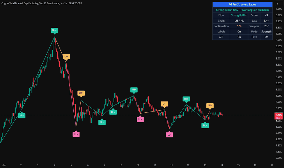
Atlantium Gold Ultra🚀 Strategy Overview: Atlantium Gold Ultra
Atlantium Gold Ultra is a quantitative trading strategy optimized for capturing mid-to-long-term market trends while maintaining a strict focus on capital preservation. The backtesting results from 2024 to early 2026 demonstrate a consistent upward equity curve with remarkable resilience during market shifts.
📊 Key Performance Metrics
Net Profit: +38.92% ($3,892.21 USD).
Profit Factor: 1.747 (Signifying a strong statistical edge).
Max Drawdown: Only 3.49% ($435.03 USD). This reflects an exceptionally conservative risk profile.
Win Rate: 44.21% (149/337 trades).
Analysis: While the win rate is below 50%, the Profit Factor of 1.747 confirms a high Risk:Reward ratio, where winning trades significantly outweigh losing ones.
🧠 Core Philosophy
The strategy is built on the principle of "cutting losses short and letting winners run." Instead of trying to predict every market micro-movement, it utilizes trend-following logic and volatility filters to ensure entries occur only during high-probability setups.
The most standout feature is the Calmar Ratio (the relationship between return and drawdown). With a return of nearly 40% against a tiny 3.49% drawdown, this strategy is ideal for traders looking for low-stress automation or those managing funded accounts.
🛠 Technical Highlights
Trend Resilience: The equity curve shows an acceleration in performance throughout 2025 and 2026, indicating the strategy thrives in trending environments.
Efficient Recovery: Drawdown periods are shallow and recovery factors are high, minimizing the time the account spends in "the red."
Trade Frequency: With 337 trades over approximately two years, the sample size is statistically significant, reducing the likelihood of "curve fitting."
📈 Suggested Description for TradingView
"I am releasing Atlantium Gold Ultra as an open-source tool for the community. This strategy focuses on trend-following with a heavy emphasis on risk management. By keeping the maximum drawdown under 4%, it provides a stable growth path even during volatile periods. Optimized for , it is designed to be a robust component of a diversified trading portfolio."
Tip for your post: Since the win rate is 44%, make sure to emphasize that the strategy relies on positive expectancy rather than high accuracy. In the trading world, a low drawdown like yours (3.49%) usually gets a lot of "Boosts" and attention! ストラテジー

インジケーター
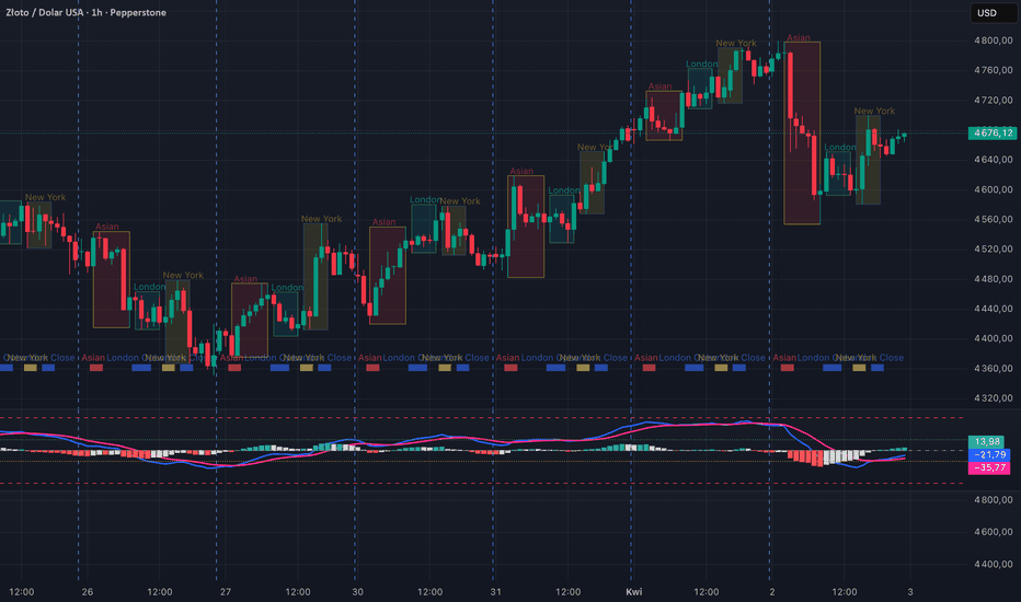
インジケーター

Vortex Nexus Alpha [JOAT]Vortex Nexus Alpha Strategy
Introduction
The Vortex Nexus Alpha Strategy is an advanced open-source algorithmic trading system that combines multi-dimensional signal generation, adaptive regime detection, and institutional-grade risk management into a unified execution framework. This strategy represents a complete trading system built from the ground up using proprietary mathematical models, fractal analysis, momentum tracking, and market microstructure intelligence.
Unlike simple crossover strategies or single-indicator systems, Vortex Nexus Alpha synthesizes intelligence from five independent signal layers, each containing five distinct detection mechanisms, creating a 25-factor confluence scoring system that validates every trade entry. The strategy is designed for traders who understand that consistent profitability requires multi-dimensional analysis, adaptive positioning, and systematic risk management rather than relying on any single indicator or pattern.
Why This Strategy Exists
This strategy addresses the fundamental challenge of algorithmic trading: most systems over-optimize to historical data or rely on simplistic logic that fails in real market conditions. Vortex Nexus Alpha solves this through a knowledge-based architecture that doesn't depend on indicator mashups but instead builds intelligence from first principles:
Volatility Expansion Engine: Measures market volatility through ATR percentile ranking and adapts position sizing and stop distances dynamically
Price Efficiency Calculator: Quantifies how efficiently price moves using path length analysis, filtering choppy conditions
Chaos Measurement System: Identifies market regime (directional, equilibrium, chaotic) using logarithmic range analysis
Directional Conviction Tracker: Measures trend strength through ADX and directional movement indicators
Adaptive Ribbon System: Multi-layer EMA ribbon that expands/contracts based on volatility and provides dynamic support/resistance
Volume Pressure Analysis: Estimates buying/selling pressure through candle structure and wick analysis
Gauss Smoothing Engine: 4th-order Gaussian filter that eliminates noise while preserving genuine price movements
Fractal Efficiency Measurement: Logarithmic efficiency calculation that adapts Laguerre filtering for optimal lag reduction
Laguerre Momentum Transform: Adaptive momentum oscillator that responds faster during efficient moves
Temporal Flow Dynamics: Analyzes price flow direction, magnitude, and acceleration across multiple dimensions
Pivot Structure Analysis: Detects market structure breaks and shifts using swing high/low analysis
Order Block Detection: Identifies institutional positioning zones through volume-confirmed reversal patterns
Imbalance Zone Mapping: Marks price gaps and inefficiencies that often get filled
Each component contributes unique intelligence that validates or invalidates potential trade setups. The strategy requires minimum confluence scores before entering positions, ensuring that multiple independent systems agree on directional bias.
Core Strategy Architecture
1. Volatility Expansion Engine
The strategy begins with comprehensive volatility analysis:
volatility = ta.atr(volatilityPeriod)
volatilityPercent = (volatility / close) * 100
volatilityRank = ta.percentrank(volatilityPercent, 100)
Volatility percentile ranking provides context for current volatility relative to recent history. This measurement drives multiple strategy decisions:
- Position sizing: Higher volatility = smaller positions
- Stop distance: Higher volatility = wider stops
- Signal filtering: Extreme volatility (>80 percentile) triggers defensive mode
The strategy adapts to volatility rather than using fixed parameters, ensuring it remains relevant across different market regimes.
2. Price Efficiency and Chaos Measurement
The strategy calculates price efficiency to distinguish trending from ranging markets:
priceMovement = math.abs(close - close )
pathLength = math.sum(math.abs(close - close ), efficiencyPeriod)
efficiency = pathLength > 0 ? priceMovement / pathLength : 0
High efficiency (>0.6) indicates clean, directional movement suitable for trend-following. Low efficiency (<0.4) suggests choppy conditions where the strategy reduces activity or switches to mean-reversion logic.
Chaos level is measured using logarithmic range analysis:
rangeHigh = ta.highest(high, volatilityPeriod)
rangeLow = ta.lowest(low, volatilityPeriod)
atrSum = math.sum(ta.atr(1), volatilityPeriod)
chaosLevel = 100 * math.log10(atrSum / (rangeHigh - rangeLow)) / math.log10(volatilityPeriod)
High chaos (>60) triggers defensive positioning. Low chaos (<40) enables aggressive trend-following.
3. Directional Conviction System
The strategy implements complete ADX analysis with directional indicators:
= adx(14, 14)
ADX above 25 indicates emerging directional conviction. Above 40 indicates dominant conviction. The strategy uses conviction strength to:
- Filter entries: Minimum conviction threshold prevents trading in directionless markets
- Size positions: Higher conviction = larger positions (within risk limits)
- Set targets: Strong conviction enables wider profit targets
The difference between bullForce and bearForce determines directional bias and validates signal direction.
4. Adaptive Ribbon System
The strategy calculates 8 EMA layers with adaptive spacing:
stepSize = (slowPeriod - fastPeriod) / (ribbonLayers - 1)
ribbonLevel0 = ta.ema(close, fastPeriod)
ribbonLevel7 = ta.ema(close, slowPeriod)
Ribbon analysis provides:
- Trend direction: Fast > slow = bullish, fast < slow = bearish
- Trend strength: Wider ribbon = stronger trend
- Dynamic support/resistance: Ribbon layers act as price magnets
- Compression detection: Tight ribbon = energy buildup before breakout
The strategy only takes long trades when price is above the ribbon and short trades when below, ensuring alignment with trend structure.
5. Volume Pressure Analysis
The strategy estimates buying and selling pressure using candle structure:
buyPressure = close > open ? volume * ((close - open + upperWick * 0.5) / barSpan) :
close < open ? volume * ((upperWick + bodyMass * 0.3) / barSpan) : volume * 0.5
sellPressure = volume - buyPressure
pressureDelta = buyPressure - sellPressure
Pressure analysis validates signal direction:
- Long signals require positive pressure delta
- Short signals require negative pressure delta
- Extreme pressure (>70% of volume) suggests potential exhaustion
The strategy tracks cumulative pressure to identify accumulation and distribution phases.
6. Gauss Smoothing and Fractal Efficiency
The strategy applies 4th-order Gaussian filtering to eliminate noise:
gaussClose := math.pow(alpha, 4) * close +
4 * (1.0 - alpha) * nz(gaussClose ) -
6 * math.pow(1 - alpha, 2) * nz(gaussClose ) +
4 * math.pow(1 - alpha, 3) * nz(gaussClose ) -
math.pow(1 - alpha, 4) * nz(gaussClose )
Fractal efficiency is calculated using logarithmic path measurement:
fractalRatio = totalSpan > 0 ? math.log(rangeSum / totalSpan) / math.log(fractalSpan) : 0.0
fractalEfficiency = math.max(0, math.min(1, (fractalRatio + 1) / 2))
High fractal efficiency (>0.7) validates that momentum signals are backed by clean price action.
7. Laguerre Momentum Transform
The strategy uses adaptive Laguerre filtering for momentum measurement:
gamma = 0.7 * (1 - fractalEfficiency) + 0.1 * fractalEfficiency
L0 := (1 - gamma) * gaussClose + gamma * nz(L0 )
L1 := -gamma * L0 + nz(L0 ) + gamma * nz(L1 )
L2 := -gamma * L1 + nz(L1 ) + gamma * nz(L2 )
L3 := -gamma * L2 + nz(L2 ) + gamma * nz(L3 )
cu = (L0 > L1 ? L0 - L1 : 0) + (L1 > L2 ? L1 - L2 : 0) + (L2 > L3 ? L2 - L3 : 0)
cd = (L0 < L1 ? L1 - L0 : 0) + (L1 < L2 ? L2 - L1 : 0) + (L2 < L3 ? L3 - L2 : 0)
laguerreValue = cu + cd != 0 ? 100 * (cu / (cu + cd)) : 50
fractalMomentum = (laguerreValue - 50) * (1 + fractalEfficiency)
The adaptive gamma adjustment reduces lag during efficient moves and adds smoothing during choppy conditions. Fractal momentum above 20 validates bullish signals, below -20 validates bearish signals.
8. Temporal Flow Dynamics
The strategy analyzes price flow across multiple dimensions:
priceFlow = ta.ema(close, flowPeriod) - ta.ema(close, flowPeriod * 2)
flowDir = priceFlow > 0 ? 1 : -1
flowMagnitude = math.abs(priceFlow) / volatility
flowAccel = ta.change(priceFlow, 3)
Flow analysis provides:
- Flow direction: Confirms trend direction
- Flow magnitude: Measures flow strength relative to volatility
- Flow acceleration: Identifies momentum shifts
The strategy requires flow alignment with signal direction for entry validation.
9. Market Structure Analysis
The strategy tracks pivot highs and lows to identify structure breaks:
pivotTop = ta.pivothigh(high, pivotSpan, pivotSpan)
pivotBottom = ta.pivotlow(low, pivotSpan, pivotSpan)
Structure breaks occur when:
- Bullish: Price breaks above previous pivot high
- Bearish: Price breaks below previous pivot low
Structure shifts (change of character) occur when:
- Bullish: Downtrend breaks above previous pivot high
- Bearish: Uptrend breaks below previous pivot low
The strategy gives bonus confluence points to signals that align with structure breaks or shifts.
10. Order Block and Imbalance Detection
The strategy identifies institutional positioning zones:
orderBlockBull = close < open and close > open and volume > avgVol * 1.2
orderBlockBear = close > open and close < open and volume > avgVol * 1.2
gapUp = low > high and (low - high ) > volatility * 0.3
gapDown = high < low and (low - high) > volatility * 0.3
Order blocks mark zones where institutions placed large orders. The strategy uses these as:
- Entry zones: Look for entries near order blocks in trend direction
- Stop placement: Place stops beyond order blocks for protection
- Target zones: Opposite-direction order blocks become profit targets
Imbalance zones (gaps) often get filled, providing mean-reversion opportunities.
Multi-Dimensional Signal Generation
The strategy generates signals through five independent layers, each containing five detection mechanisms:
Layer 1: Rapid Scalp Signals (5 mechanisms)
- Laguerre oversold + flow bullish + price above fast ribbon
- Pressure index positive + flow reversal bullish
- Momentum bullish + volume surge + price above mid ribbon
- Strong bullish candle + ribbon bullish + pressure positive
- Fractal momentum positive + flow acceleration positive + ribbon aligned
Layer 2: Swing Position Signals (5 mechanisms)
- Ribbon bullish + price above slow ribbon + bullish regime
- Structure break bullish + momentum bullish
- Order block bullish + flow bullish + conviction strong
- Gap up + pressure extreme + ribbon aligned
- Range breakout up + cumulative pressure positive + flow strong
Layer 3: Momentum Continuation (5 mechanisms)
- Fractal momentum extreme + ribbon bullish + conviction strong
- Laguerre oversold + flow bullish + volume surge
- Momentum extreme + fractal momentum positive + ribbon expanding
- Extreme buy pressure + flow acceleration positive + bullish regime
- Bull force > bear force + conviction strong + ribbon aligned
Layer 4: Structure Confirmation (5 mechanisms)
- Structure shift bullish + volume surge
- Order block bullish + price above last pivot low + momentum bullish
- Gap up + flow bullish + ribbon bullish
- Structure break bullish + pressure extreme positive
- Volume absorption + pressure positive + price above mid ribbon
Layer 5: Confluence Boosters (5 mechanisms)
- Ribbon tight + ribbon expanding + ribbon bullish + volume surge
- Net flow positive + temporal force positive + bullish regime
- Fractal efficiency high + Laguerre oversold + flow magnitude strong
- Strong bullish candle + price above previous high + volume extreme
- Velocity positive + flow bullish + ribbon power strong
Each layer contributes 0 or 1 to the bull strength score. The strategy requires minimum confluence (default 2) before entering long positions. This multi-layer approach ensures that signals are validated across multiple independent dimensions.
Risk Management System
The strategy implements institutional-grade risk management:
Position Sizing:
- Risk percentage per trade (default 1% of equity)
- Dynamic adjustment based on volatility percentile
- Reduced sizing during high chaos or low efficiency
Stop Loss Placement:
stopLoss = close - (volatility * slMultiplier)
- ATR-based stops that adapt to current volatility
- Multiplier (default 1.5) provides breathing room
- Stops placed beyond order blocks when possible
Take Profit Targets:
takeProfit = close + (volatility * slMultiplier * tpMultiplier)
- Risk-reward ratio (default 2.5:1)
- Adjusted based on conviction strength
- Wider targets during strong conviction, tighter during weak
Trailing Stop System:
trailStop = close - (volatility * trailOffset)
- Optional trailing stop (default enabled)
- Offset (default 1.2x ATR) balances protection and breathing room
- Activates after position moves into profit
Visual Elements
Adaptive Ribbon: Multi-layer EMA ribbon with gradient coloring showing trend direction and strength
Entry Signals: Triangle shapes sized by signal strength (large for 5+ confluence, small for 2-3 confluence)
Structure Markers: Lines and labels marking structure breaks, shifts, and order blocks
Imbalance Boxes: Boxes marking price gaps and inefficiency zones
Regime Background: Subtle background coloring showing current market regime
Flow Background: Additional background layer showing flow direction
Comprehensive Dashboard: 18-row intelligence panel showing position status, signal strength, regime, ribbon state, pressure, momentum, structure, flow, conviction, Laguerre, volume, volatility, trade statistics, and win rate
The dashboard provides complete strategy intelligence with real-time metrics and performance tracking.
Strategy Parameters
Core Settings:
Ultra-Aggressive Mode: Maximum trade frequency (default enabled)
Min Signal Strength: Minimum confluence required (1-6, default 2)
Risk %: Risk per trade as percentage of equity (0.5-5.0%, default 1.0%)
TP Multiplier: Take profit as multiple of stop distance (1.0-10.0, default 2.5)
SL Multiplier: Stop loss as multiple of ATR (0.5-5.0, default 1.5)
Trailing Stop: Enable/disable trailing stop (default enabled)
Trail Offset: Trailing stop distance as multiple of ATR (0.5-3.0, default 1.2)
Advanced Parameters:
Volatility Period: ATR calculation length (5-50, default 14)
Efficiency Period: Price efficiency calculation period (5-100, default 20)
Flow Period: Temporal flow analysis period (10-50, default 20)
Ribbon Layers: Number of EMA layers (3-15, default 8)
Fast Period: Fastest EMA period (2-20, default 5)
Slow Period: Slowest EMA period (10-100, default 34)
Visualization:
Dashboard: Toggle metrics panel (default enabled)
Entry Signals: Toggle signal shapes (default enabled)
Regime Zones: Toggle background coloring (default enabled)
Adaptive Ribbon: Toggle ribbon display (default enabled)
How to Use This Strategy
Step 1: Configure Risk Parameters
Set risk percentage appropriate for your account size. 1% is conservative, 2% is moderate, 3%+ is aggressive. Never risk more than you can afford to lose on any single trade.
Step 2: Select Minimum Signal Strength
Default 2 provides balanced trade frequency and quality. Increase to 3-4 for higher quality but fewer trades. Decrease to 1 only in ultra-aggressive mode on highly liquid instruments.
Step 3: Adjust Risk-Reward Ratio
Default 2.5:1 provides good balance. Increase to 3-5:1 for swing trading. Decrease to 1.5-2:1 for scalping. Higher ratios require higher win rates to be profitable.
Step 4: Enable/Disable Trailing Stops
Trailing stops protect profits but can exit prematurely. Enable for trend-following, disable for mean-reversion. Adjust trail offset based on instrument volatility.
Step 5: Monitor Dashboard Metrics
Watch "POSITION" status, "BULL STR" and "BEAR STR" scores, "REGIME" classification, and "WIN RATE" percentage. These provide real-time strategy health assessment.
Step 6: Backtest Thoroughly
Test on at least 100 trades across different market conditions. Verify that win rate, profit factor, and drawdown meet your requirements. Adjust parameters if needed.
Step 7: Forward Test on Demo
Run strategy on demo account for at least 1 month before live trading. Verify that live performance matches backtest expectations. Monitor slippage and execution quality.
Step 8: Start Small on Live
Begin with minimum position sizes on live account. Gradually increase as confidence builds. Never risk more than 1-2% of account on any single trade initially.
Best Practices
Use on liquid instruments with tight spreads and reliable execution
Backtest with realistic commission (0.1%) and slippage (2 ticks minimum)
Test across multiple market conditions (trending, ranging, volatile, calm)
Verify minimum 100 trades in backtest for statistical significance
Monitor win rate - should be 45-60% for 2.5:1 risk-reward ratio
Check profit factor - should be >1.5 for robust strategy
Analyze maximum drawdown - should be <20% of account
Review trade distribution - avoid over-concentration in specific periods
Monitor signal strength distribution - most trades should be 3+ confluence
Check regime alignment - strategy should perform in directional regimes
Verify that losses are controlled - no single loss should exceed 2% of account
Ensure adequate trade frequency - at least 2-3 trades per week on daily timeframe
Combine with manual oversight - review signals before execution in early stages
Use appropriate timeframe - 15m-1H for day trading, 4H-1D for swing trading
Avoid trading during major news events unless specifically tested for that
Keep detailed trade journal to identify patterns in wins and losses
Strategy Limitations
Algorithmic strategies cannot predict black swan events or unprecedented market conditions
Backtested performance does not guarantee future results
Slippage and commission in live trading may differ from backtest assumptions
The strategy requires sufficient volatility - may underperform in extremely low volatility
Signal generation depends on multiple calculations - computational lag possible on slow systems
The strategy works best on trending instruments - may struggle in perpetual ranges
Confluence scoring requires all components to be relevant - some may be less meaningful on certain instruments
The strategy cannot account for fundamental catalysts or news events
Trailing stops can exit prematurely during volatile but ultimately profitable moves
The strategy requires adequate liquidity for execution at desired prices
Parameter optimization can lead to overfitting - use walk-forward analysis
The strategy shows what signals exist, not why - market context still matters
Technical Implementation
Built with Pine Script v6 using:
Complete volatility expansion engine with ATR percentile ranking
Price efficiency calculator using path length analysis
Chaos measurement using logarithmic range calculations
Full ADX implementation with directional indicators
8-layer adaptive EMA ribbon with volatility-based spacing
Volume pressure estimation using candle structure analysis
4th-order Gaussian filter for noise elimination
Fractal efficiency measurement using logarithmic path complexity
Adaptive Laguerre transform with 4 cascading filter levels
Temporal flow analysis with direction, magnitude, and acceleration
Pivot-based market structure tracking
Order block and imbalance zone detection
25-factor confluence scoring system across 5 signal layers
Dynamic position sizing based on volatility and regime
ATR-based stop loss and take profit calculations
Optional trailing stop system with volatility adjustment
Comprehensive dashboard with 18 metrics and performance tracking
Alert system for all entry and exit signals
The code is fully open-source with extensive comments explaining each component and signal generation logic.
Originality Statement
This strategy is original and represents a complete trading system built from proprietary knowledge rather than indicator mashups. The strategy is justified because:
It synthesizes 13 independent analytical systems into a unified execution framework
The 25-factor confluence scoring across 5 signal layers provides multi-dimensional validation
Each component is built from first principles using mathematical models and market microstructure concepts
The adaptive nature of the system (volatility, efficiency, regime) ensures relevance across market conditions
Risk management is integrated at the core rather than added as an afterthought
The strategy doesn't rely on any single indicator or pattern - it builds intelligence from multiple independent sources
Fractal efficiency and Laguerre adaptation provide unique momentum measurement not found in standard systems
Temporal flow analysis adds a dimension of price dynamics beyond simple trend following
Market structure tracking provides context that pure indicator-based systems lack
The comprehensive dashboard provides complete strategy intelligence and performance tracking
The system is designed for real trading with realistic risk management, not just backtest optimization
Each component contributes unique intelligence: volatility drives adaptation, efficiency filters conditions, chaos identifies regimes, conviction measures strength, ribbon provides structure, pressure shows order flow, Gauss filtering eliminates noise, fractal efficiency validates momentum, Laguerre provides adaptive momentum, flow tracks dynamics, structure provides context, order blocks mark zones, and confluence validates signals. The strategy's value lies in combining these complementary perspectives into a cohesive, adaptive trading system with institutional-grade risk management.
Disclaimer
This strategy is provided for educational and informational purposes only. It is not financial advice or a recommendation to buy or sell any financial instrument. Trading involves substantial risk of loss and is not suitable for all investors.
Algorithmic trading strategies are tools for systematic execution, not guarantees of profit. Backtested performance does not guarantee future results. Past strategy performance does not predict future performance. Market conditions change, and strategies that worked historically may not work in the future.
The signals generated are mathematical calculations based on current market data, not predictions of future price movement. High confluence scores, regime alignment, and structure breaks do not guarantee profitable trades. Users must conduct their own analysis and risk assessment before making trading decisions.
Always use proper risk management, including stop losses and position sizing appropriate for your account size and risk tolerance. Never risk more than you can afford to lose. Consider consulting with a qualified financial advisor before making investment decisions.
The author is not responsible for any losses incurred from using this strategy. Users assume full responsibility for all trading decisions made using this tool. Thoroughly backtest and forward test any strategy before live trading.
-Made with passion by officialjackofalltrades ストラテジー

SMC EMA CROSS ZIG ZAG# Mega Trend Suite – SMC + EMA (Lightweight Edition)
**A professional Smart Money Concepts (SMC) toolkit combined with classic EMA crossovers and VWAP.**
No Heikin Ashi, no MA Cross EMA – just clean price action, order flow, and trend confirmation.
---
## 🔍 Overview
This indicator bundles the most essential tools for **institutional-style analysis**:
- ✅ **SMC Structure** (internal & swing BOS/CHoCH)
- ✅ **Order Blocks** (bullish/bearish, with box or candle highlight)
- ✅ **Fair Value Gaps (FVG)** with auto threshold & multi‑timeframe support
- ✅ **Premium / Discount Zones** + Equilibrium line
- ✅ **Multi‑Timeframe High/Low levels** (Daily / Weekly / Monthly)
- ✅ **ZigZag** (main & internal) with HH/HL/LH/LL labels
- ✅ **VWAP** – anchored to the session
- ✅ **Two EMA sets** (9/21 & 20/50) with cross signals
- ✅ **Compact Dashboard** (SMC bias & current timeframe)
- ✅ **Full alert system** for all SMC events and EMA crosses
---
## 🧠 Key Features Explained
### 1. Smart Money Concepts (SMC)
| Component | What it does |
|-----------|---------------|
| **Swing Structure** | Detects Break of Structure (BOS) and Change of Character (CHoCH) on a higher‑length pivot (default 50). Shows labels “BOS” or “CHoCH” when price crosses a swing high/low. |
| **Internal Structure** | Same as swing, but uses a shorter length (default 10) to catch micro‑structure changes. Optional confluence filter (body vs. wick). |
| **Order Blocks (OB)** | Stores the extreme bar (parsed by volatility filter) after a valid BOS/CHoCH. Displays as zone boxes or candle highlights. Mitigation detection (close / high/low). |
| **Fair Value Gaps (FVG)** | Detects 3‑bar imbalances on a chosen timeframe (or current). Uses auto‑threshold based on historical bar delta. Extendable boxes. |
| **Premium / Discount Zones** | Calculates the range between the highest swing high and lowest swing low. Shades the upper 50% (premium) and lower 50% (discount) with an equilibrium line in the middle. |
| **MTF High/Low Levels** | Plots previous period’s high/low for Daily, Weekly, Monthly. Line style (solid/dashed/dotted) and color customizable. |
| **ZigZag** | Classic pivot‑based ZigZag with HH/HL/LH/LL labels. Separate internal ZigZag available for finer swings. |
### 2. VWAP
- Standard Volume Weighted Average Price.
- Useful for intraday bias – price above VWAP = bullish tilt.
### 3. EMA Sets
Two independent EMA pairs:
- **Set 1:** 9 & 21 (fast)
- **Set 2:** 20 & 50 (slower)
Each set plots its own lines and generates up/down triangles on crossover / crossunder. Colours, widths, and signal colours are fully adjustable.
---
## ⚙️ Input Parameters (Grouped)
### 🔧 Master Controls
- `Enable SMC Module` – turn all SMC features on/off.
### 📊 SMC – General
- `Mode` – Historical (keeps all drawings) / Present (refreshes each bar).
- `Style` – Colored / Monochrome.
### 📊 SMC – Structure & Order Blocks
- Internal / Swing lengths, label sizes, BOS/CHoCH filter (All / BOS only / CHoCH only).
- OB display mode (Both / Zone Box / Candle Highlight).
- OB mitigation source (Close / High/Low).
- OB filter (ATR / Cumulative Mean Range).
### 📊 SMC – Fair Value Gaps
- Auto threshold on/off, custom timeframe, extend bars.
### 📊 SMC – MTF High/Low Levels
- Show Daily / Weekly / Monthly – each with independent line style & colour.
### 📊 SMC – Premium / Discount Zones
- Toggle zones, custom colours for premium, equilibrium, discount.
### 📊 ZigZag Swing Lines
- Main ZigZag depth/deviation/backstep, colours, width, style, labels.
- Optional internal ZigZag with separate settings.
### 📈 VWAP & EMA Sets
- VWAP on/off, colour, width.
- Two EMA sets: each with fast/slow lengths, colours, line width, cross signal colours.
### 📊 Dashboard
- Position (Top‑Left/Right, Bottom‑Left/Right), font size.
### 🎨 Colors
- Global bull / bear / neutral colours (used in dashboard).
---
## 🖥️ Dashboard
A small table shows at a glance:
- **SMC Bias** – Bullish / Bearish / Neutral (based on swing trend).
- **Current Timeframe** – e.g., “60” for 1h, “D” for daily.
The dashboard adapts to dark/light chart background.
---
## 🚨 Alerts (30+ conditions)
All alerts are available from the TradingView alert dialog:
| Category | Alerts |
|----------|--------|
| **Internal Structure** | Bull/Bear BOS, Bull/Bear CHoCH |
| **Swing Structure** | Bull/Bear BOS, Bull/Bear CHoCH |
| **Order Blocks** | Bull/Bear Internal OB mitigated, Bull/Bear Swing OB mitigated |
| **Fair Value Gaps** | Bull FVG formed, Bear FVG formed |
| **EMA Crosses** | EMA Set 1/2 Bull Cross, Bear Cross |
---
## 🧩 How to Use
1. **Add the indicator** to any chart (any symbol, any timeframe).
2. **Keep default settings** for a clean SMC + EMA experience.
3. **For scalping / intraday:**
- Enable Internal Structure (length 5–10).
- Use VWAP as bias filter.
- Watch for FVGs on 1m–15m.
4. **For swing trading:**
- Focus on Swing Structure (length 50+).
- Use Premium/Discount zones for entries (buy in discount, sell in premium).
- Confirm with EMA Set 2 (20/50) cross.
5. **Order Blocks:**
- When price returns to a bullish OB zone, look for buying opportunities.
- When a bearish OB gets mitigated, expect continuation down.
---
## 💡 Tips
- **Monochrome style** is perfect for grayscale / minimalistic setups.
- **Present mode** keeps drawings only on the current visible bars – useful for low‑resource usage.
- **FVG auto‑threshold** works best on higher timeframes (1h+). For lower timeframes, you may turn it off and use manual threshold via the `barDelta` calculation (already built‑in).
- The **ZigZag** does not repaint – it uses confirmed pivots.
---
## 📜 Credits & Version
- **Original concept:** Mega Trend Suite (SMC + HAMA + MA Cross EMA)
- **This edition:** Removed HAMA, MA Cross EMA, and Heikin Ashi Smoothed – keeping only SMC, VWAP, and EMA sets.
- **Version:** 1.0 (Pine Script v6)
---
## ❗ Notes
- This indicator is **not a financial advice** – always use proper risk management.
- Maximum drawings (labels, lines, boxes) are set to 500 each – enough for several months of data.
- Multi‑timeframe levels (Daily/Weekly/Monthly) work correctly only if the chart has enough historical data.
---
**Happy trading!**
*Mega Trend Suite – SMC + EMA* インジケーター