전략

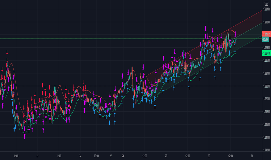
Moving Regression Prediction BandsIntroducing the Moving Regression Prediction Bands indicator.
Here I aimed to combine the principles of traditional band indicators (such as Bollinger Bands), regression channel and outlier detection methods. Its upper and lower bands define an interval in which the current price was expected to fall with a prescribed probability, as predicted by the previous-step result of the local polynomial regression (for the original Moving Regression script, see link below).
Algorithm
1. At every time step, the script performs local polynomial regression of the sample data within the lookback window specified by the Length input parameter.
2. The fitted polynomial is used to construct the Moving Regression time series as well as to extrapolate data, that is, to predict the next data point ( MRPrediction ).
3. The accuracy of local interpolation is estimated by means of the root-mean-square error ( RMSE ), that is, the deviation between the fitted polynomial and the observed values.
4. The MRPrediction and RMSE values calculated for the previous bar are then used to build the upper and lower bands , which I define as follows:
Upper Band = MRPrediction_prev + Multiplier *( RMSE_prev )
Lower Band = MRPrediction_prev - Multiplier *( RMSE_prev )
Here the Multiplier is a user-defined parameter that should be interpreted as a quantile in the standard normal distribution (the default value of 2.0 roughly corresponds to the 95% prediction interval).
To visualize the central line , the script offers the following options:
Previous-Period MR Prediction: MRPrediction_prev time series from the above equation.
MR: Conventional Moving Regression time series.
Ribbon: “Previous-Period MR Prediction” and “MR” curves plotted together and colored according to their relative value (green if MR > Previous MR Prediction; red otherwise).
Usage
My original idea was to use the band breakouts as potential trading signals. For example, the price crossing above the upper band is a bullish signal , being a potential sign that price is gaining momentum and is out of a previously predicted trend. The exit signal could be the crossing under the lower band or under the central line.
However, be aware that it is an experimental indicator, so you might fin some better strategies.
Feel free to play around!
지표

Nico's SPX Dynamic ChannelsTest of dynamic channels and some statistics made by hand.
This indicator was done specifically for the S&P500 index.
As you can see, below the 125 EMA there's a lot more volatility than in the upside. I've made some kind of a dynamic linear regression of the lows and the highs.
I've chosen the MA that best fits the SPX, and then calculated in Excel the percental mean and SDs of most important peaks and valleys that I've chosen in comparison to the 125 MA. This lead to the green, orange and red zones. BUT, I've calculated the peaks and valleys separately, as I assumed that a bear market and crashes have way more volatility than bull markets. That's why the difference between the upper and the lower channels.
The neutral blue zone is composed by an upper EMA of the highs and lower EMA of the lows. No MA in this script uses the close price as a source.
This MA makes sense because it represents a semester of trading, for this particular asset.
Backtest results
It's also interesting to try it here too, as it has a little bit more of data:
SPCFD:SPX
As it's not a trading system, I have no batting average nor ratios for this.
Still, the measures of the peaks and valleys are very accurate and repeat themselves over and over again. The results were:
3rd resistance: 12.88%
2nd resistance: 10.12%
1st resistance: 7.36%
1st support: -6.42%
2nd support: -14.8%
3rd support: -23.18%
All referred to the mean, which is the 125 EMA zone.
After the 1950's works like magic, but not before. You will see that it doesn't work in the great depression and it's crash.
How to use this indicator
Green = First grade support/resistance .
Orange = Second grade support/resistance . Caution.
Red = Third grade support/resistance . High chances of mean reversal.
Blue zone = This is the neutral zone, where the prices are not cheap nor expensive.
Often in a trending market, the price will have the blue zone as it's main support and when trending the price will stick to the green MA.
When the price touches the orange MA, the most probable is that it will return to the green MA.
If the price touches the red zone, there's a high chance that this is a big turning point and it will reverse to the mean (green or blue zone).
Imagine you've bought each time the price touched the red support, check that and you'll start liking this indicator. I think it is a great entry point for investors. The red resistance is good too, but of course it works for a short period of time.
I've backtested this indicator since the beginning of the dataset and it works like magic, but ONLY for the SPX index (spot price).
Leave a comment or some coins if you like it!!!
(I've posted it before like an analysis, not as a script, my bad) 지표

지표

지표
Theil–Sen EstimatorThe Theil-Sen estimator is a nonparametric statistics method for robustly fitting a regression line to sample points (1,2).
As stated in the Wikipedia article (3), the method is " the most popular nonparametric technique for estimating a linear trend " in the applied sciences due to its robustness to outliers and limited assumptions regarding measurement errors.
Relation with other Methods
The Theil-Sen estimator can be significantly more accurate than simple linear regression (least squares) for skewed and heteroskedastic data.
Method Description
The script computes all the slopes between pairs of points and takes the median as the estimate of the regression slope, m . Subsequently, the intercept, b , is determined from the sample points as the median of y(i) − m x(i) values. The regression line in the slope–intercept form, y = m x + b , is then plotted along with the calculated prediction interval (estimated by means of the root-mean-square error).
I have added two options for how to handle pairs of points:
Method == "All" to use the slopes of all pairs of points;
Method == "Random" to use the slopes of randomly generated pairs of points.
The random choice of the pairs of points is based on the Wichmann–Hill is a pseudorandom number generator.
The reason for introducing the "Random" method is that the calculation of the median involves sorting the array of slopes (the size of N*(N-1)/2, where N is the number of sample points). This is a computationally demanding procedure, which runs into the limit on the cycle computation time (200 ms) set in TradingView. Therefore, the "All" method works only with Length < 50.
Also note that the number of lookback points is limited by by the maximum array size allowed in TradingView.
Literature
1. Sen, P. K. (1968) "Estimates of the regression coefficient based on Kendall's tau." JASA, 1379-1389.
2. Theil, H. (1950) "A rank-invariant method of linear and polynomial regression analysis." Reprinted in 1992 in Henri Theil’s contributions to economics and econometrics, Springer, 345-381.
3. en.wikipedia.org 지표

지표

지표

지표

Moving RegressionMoving Regression is a generalization of moving average and polynomial regression.
The procedure approximates a specified number of prior data points with a polynomial function of a user-defined degree. Then, polynomial interpolation of the last data point is used to construct a Moving Regression time series.
Application:
Moving Regression allows one to smooth noise on the analyzed chart, assess momentum, confirm trends, and establish areas of support and resistance.
In addition, it can be used as a simple stand-alone forecasting method to identify trend direction and trend reversal points. When the local polynomial is predicted to move up in the next time step, the color of the Moving Regression curve will be green. Otherwise, the color of the curve is red. This function is (de)activated using the Predict Trend Direction flag.
Selecting the model parameters:
The effects of the moving window Length and the Local Polynomial Degree are confounded. This allows for finding the optimal trade-off between noise (variance) and lag (bias). Higher Length and lower Polynomial Degree (such as 1, i.e. linear), will result in "smoother" time series but at the cost of greater lag. Increasing the Polynomial Degree to, for example, 2 (squared) while maintaining the Length will diminish the lag and thus compromise the noise-lag tradeoff.
Relation to other methods:
When the degree of the local polynomial is set to 0 (i.e., fitting data to a constant level), the Moving Regression time series exactly matches the Simple Moving Average of the same length. 지표

전략
지표

지표

지표

지표

지표

지표

지표

Donchian BlasterRelease Note:
Keeping in mind of getting full potential of Donchian Channels, As part of this script, Linear Regression is used as primary source to identify trend and execute the trades.
Hull Moving Average given as alternative option in place of Linear regression.
Linear Regression:
Linear regression used to identify trend, trade setup, and stop. Based on this, Color fillings on Donchian channels is updated. That will give clear idea of strength or weakness in any trading instruments.
HMA:
HMA used as alternative to identify trend, trade setup, and stop. Based on this, Color fillings on Donchian channels is updated. That will give clear idea of strength or weakness in any trading instruments.
Donchian Channels:
As it is one of the oldest trend riding system, combined here with differentiation in color will help to go with the trend.
Inputs:
Input periods can be changed by users/traders as per their understanding and observations.
//Disclaimer: Idea of publishing this script is to identify the strength of the instrument using multiple confirmation.
//Disclaimer: Using this indicator, changing inputs, and trading decisions are up to the users/traders.
//Courtesy: Thanks to Richard Donchian, Alan Hull, and author of LSMA as this indicator/script inspired by Donchian Channels, Hull Moving Average, and LSMA 지표

지표

지표
지표

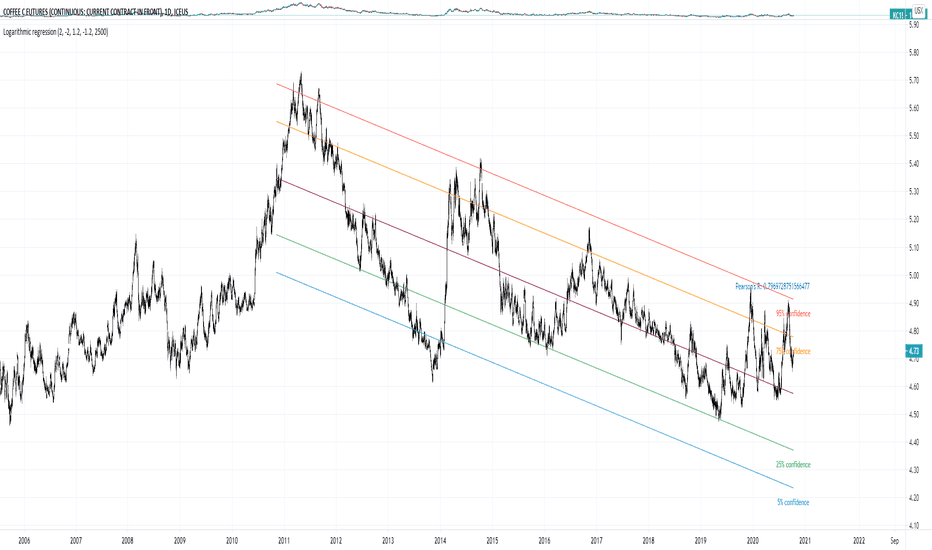
Polynomial Regression Bands + Channel [DW]This is an experimental study designed to calculate polynomial regression for any order polynomial that TV is able to support.
This study aims to educate users on polynomial curve fitting, and the derivation process of Least Squares Moving Averages (LSMAs).
I also designed this study with the intent of showcasing some of the capabilities and potential applications of TV's fantastic new array functions.
Polynomial regression is a form of regression analysis in which the relationship between the independent variable x and the dependent variable y is modeled as a polynomial of nth degree (order).
For clarification, linear regression can also be described as a first order polynomial regression. The process of deriving linear, quadratic, cubic, and higher order polynomial relationships is all the same.
In addition, although deriving a polynomial regression equation results in a nonlinear output, the process of solving for polynomials by least squares is actually a special case of multiple linear regression.
So, just like in multiple linear regression, polynomial regression can be solved in essentially the same way through a system of linear equations.
In this study, you are first given the option to smooth the input data using the 2 pole Super Smoother Filter from John Ehlers.
I chose this specific filter because I find it provides superior smoothing with low lag and fairly clean cutoff. You can, of course, implement your own filter functions to see how they compare if you feel like experimenting.
Filtering noise prior to regression calculation can be useful for providing a more stable estimation since least squares regression can be rather sensitive to noise.
This is especially true on lower sampling lengths and higher degree polynomials since the regression output becomes more "overfit" to the sample data.
Next, data arrays are populated for the x-axis and y-axis values. These are the main datasets utilized in the rest of the calculations.
To keep the calculations more numerically stable for higher periods and orders, the x array is filled with integers 1 through the sampling period rather than using current bar numbers.
This process can be thought of as shifting the origin of the x-axis as new data emerges.
This keeps the axis values significantly lower than the 10k+ bar values, thus maintaining more numerical stability at higher orders and sample lengths.
The data arrays are then used to create a pseudo 2D matrix of x power sums, and a vector of x power*y sums.
These matrices are a representation the system of equations that need to be solved in order to find the regression coefficients.
Below, you'll see some examples of the pattern of equations used to solve for our coefficients represented in augmented matrix form.
For example, the augmented matrix for the system equations required to solve a second order (quadratic) polynomial regression by least squares is formed like this:
(∑x^0 ∑x^1 ∑x^2 | ∑(x^0)y)
(∑x^1 ∑x^2 ∑x^3 | ∑(x^1)y)
(∑x^2 ∑x^3 ∑x^4 | ∑(x^2)y)
The augmented matrix for the third order (cubic) system is formed like this:
(∑x^0 ∑x^1 ∑x^2 ∑x^3 | ∑(x^0)y)
(∑x^1 ∑x^2 ∑x^3 ∑x^4 | ∑(x^1)y)
(∑x^2 ∑x^3 ∑x^4 ∑x^5 | ∑(x^2)y)
(∑x^3 ∑x^4 ∑x^5 ∑x^6 | ∑(x^3)y)
This pattern continues for any n ordered polynomial regression, in which the coefficient matrix is a n + 1 wide square matrix with the last term being ∑x^2n, and the last term of the result vector being ∑(x^n)y.
Thanks to this pattern, it's rather convenient to solve the for our regression coefficients of any nth degree polynomial by a number of different methods.
In this script, I utilize a process known as LU Decomposition to solve for the regression coefficients.
Lower-upper (LU) Decomposition is a neat form of matrix manipulation that expresses a 2D matrix as the product of lower and upper triangular matrices.
This decomposition method is incredibly handy for solving systems of equations, calculating determinants, and inverting matrices.
For a linear system Ax=b, where A is our coefficient matrix, x is our vector of unknowns, and b is our vector of results, LU Decomposition turns our system into LUx=b.
We can then factor this into two separate matrix equations and solve the system using these two simple steps:
1. Solve Ly=b for y, where y is a new vector of unknowns that satisfies the equation, using forward substitution.
2. Solve Ux=y for x using backward substitution. This gives us the values of our original unknowns - in this case, the coefficients for our regression equation.
After solving for the regression coefficients, the values are then plugged into our regression equation:
Y = a0 + a1*x + a1*x^2 + ... + an*x^n, where a() is the ()th coefficient in ascending order and n is the polynomial degree.
From here, an array of curve values for the period based on the current equation is populated, and standard deviation is added to and subtracted from the equation to calculate the channel high and low levels.
The calculated curve values can also be shifted to the left or right using the "Regression Offset" input
Changing the offset parameter will move the curve left for negative values, and right for positive values.
This offset parameter shifts the curve points within our window while using the same equation, allowing you to use offset datapoints on the regression curve to calculate the LSMA and bands.
The curve and channel's appearance is optionally approximated using Pine's v4 line tools to draw segments.
Since there is a limitation on how many lines can be displayed per script, each curve consists of 10 segments with lengths determined by a user defined step size. In total, there are 30 lines displayed at once when active.
By default, the step size is 10, meaning each segment is 10 bars long. This is because the default sampling period is 100, so this step size will show the approximate curve for the entire period.
When adjusting your sampling period, be sure to adjust your step size accordingly when curve drawing is active if you want to see the full approximate curve for the period.
Note that when you have a larger step size, you will see more seemingly "sharp" turning points on the polynomial curve, especially on higher degree polynomials.
The polynomial functions that are calculated are continuous and differentiable across all points. The perceived sharpness is simply due to our limitation on available lines to draw them.
The approximate channel drawings also come equipped with style inputs, so you can control the type, color, and width of the regression, channel high, and channel low curves.
I also included an input to determine if the curves are updated continuously, or only upon the closing of a bar for reduced runtime demands. More about why this is important in the notes below.
For additional reference, I also included the option to display the current regression equation.
This allows you to easily track the polynomial function you're using, and to confirm that the polynomial is properly supported within Pine.
There are some cases that aren't supported properly due to Pine's limitations. More about this in the notes on the bottom.
In addition, I included a line of text beneath the equation to indicate how many bars left or right the calculated curve data is currently shifted.
The display label comes equipped with style editing inputs, so you can control the size, background color, and text color of the equation display.
The Polynomial LSMA, high band, and low band in this script are generated by tracking the current endpoints of the regression, channel high, and channel low curves respectively.
The output of these bands is similar in nature to Bollinger Bands, but with an obviously different derivation process.
By displaying the LSMA and bands in tandem with the polynomial channel, it's easy to visualize how LSMAs are derived, and how the process that goes into them is drastically different from a typical moving average.
The main difference between LSMA and other MAs is that LSMA is showing the value of the regression curve on the current bar, which is the result of a modelled relationship between x and the expected value of y.
With other MA / filter types, they are typically just averaging or frequency filtering the samples. This is an important distinction in interpretation. However, both can be applied similarly when trading.
An important distinction with the LSMA in this script is that since we can model higher degree polynomial relationships, the LSMA here is not limited to only linear as it is in TV's built in LSMA.
Bar colors are also included in this script. The color scheme is based on disparity between source and the LSMA.
This script is a great study for educating yourself on the process that goes into polynomial regression, as well as one of the many processes computers utilize to solve systems of equations.
Also, the Polynomial LSMA and bands are great components to try implementing into your own analysis setup.
I hope you all enjoy it!
--------------------------------------------------------
NOTES:
- Even though the algorithm used in this script can be implemented to find any order polynomial relationship, TV has a limit on the significant figures for its floating point outputs.
This means that as you increase your sampling period and / or polynomial order, some higher order coefficients will be output as 0 due to floating point round-off.
There is currently no viable workaround for this issue since there isn't a way to calculate more significant figures than the limit.
However, in my humble opinion, fitting a polynomial higher than cubic to most time series data is "overkill" due to bias-variance tradeoff.
Although, this tradeoff is also dependent on the sampling period. Keep that in mind. A good rule of thumb is to aim for a nice "middle ground" between bias and variance.
If TV ever chooses to expand its significant figure limits, then it will be possible to accurately calculate even higher order polynomials and periods if you feel the desire to do so.
To test if your polynomial is properly supported within Pine's constraints, check the equation label.
If you see a coefficient value of 0 in front of any of the x values, reduce your period and / or polynomial order.
- Although this algorithm has less computational complexity than most other linear system solving methods, this script itself can still be rather demanding on runtime resources - especially when drawing the curves.
In the event you find your current configuration is throwing back an error saying that the calculation takes too long, there are a few things you can try:
-> Refresh your chart or hide and unhide the indicator.
The runtime environment on TV is very dynamic and the allocation of available memory varies with collective server usage.
By refreshing, you can often get it to process since you're basically just waiting for your allotment to increase. This method works well in a lot of cases.
-> Change the curve update frequency to "Close Only".
If you've tried refreshing multiple times and still have the error, your configuration may simply be too demanding of resources.
v4 drawing objects, most notably lines, can be highly taxing on the servers. That's why Pine has a limit on how many can be displayed in the first place.
By limiting the curve updates to only bar closes, this will significantly reduce the runtime needs of the lines since they will only be calculated once per bar.
Note that doing this will only limit the visual output of the curve segments. It has no impact on regression calculation, equation display, or LSMA and band displays.
-> Uncheck the display boxes for the drawing objects.
If you still have troubles after trying the above options, then simply stop displaying the curve - unless it's important to you.
As I mentioned, v4 drawing objects can be rather resource intensive. So a simple fix that often works when other things fail is to just stop them from being displayed.
-> Reduce sampling period, polynomial order, or curve drawing step size.
If you're having runtime errors and don't want to sacrifice the curve drawings, then you'll need to reduce the calculation complexity.
If you're using a large sampling period, or high order polynomial, the operational complexity becomes significantly higher than lower periods and orders.
When you have larger step sizes, more historical referencing is used for x-axis locations, which does have an impact as well.
By reducing these parameters, the runtime issue will often be solved.
Another important detail to note with this is that you may have configurations that work just fine in real time, but struggle to load properly in replay mode.
This is because the replay framework also requires its own allotment of runtime, so that must be taken into consideration as well.
- Please note that the line and label objects are reprinted as new data emerges. That's simply the nature of drawing objects vs standard plots.
I do not recommend or endorse basing your trading decisions based on the drawn curve. That component is merely to serve as a visual reference of the current polynomial relationship.
No repainting occurs with the Polynomial LSMA and bands though. Once the bar is closed, that bar's calculated values are set.
So when using the LSMA and bands for trading purposes, you can rest easy knowing that history won't change on you when you come back to view them.
- For those who intend on utilizing or modifying the functions and calculations in this script for their own scripts, I included debug dialogues in the script for all of the arrays to make the process easier.
To use the debugs, see the "Debugs" section at the bottom. All dialogues are commented out by default.
The debugs are displayed using label objects. By default, I have them all located to the right of current price.
If you wish to display multiple debugs at once, it will be up to you to decide on display locations at your leisure.
When using the debugs, I recommend commenting out the other drawing objects (or even all plots) in the script to prevent runtime issues and overlapping displays. 지표