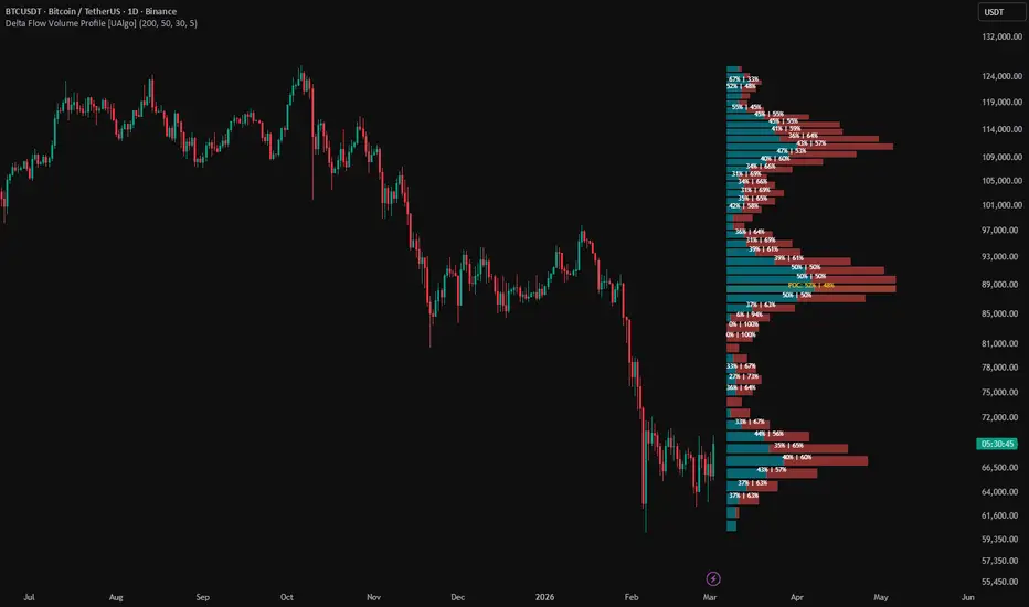
Volume Delta with Fibonacci Projection [UAlgo]Volume Delta Profile with Fibonacci Projection is a structure driven profiling tool that combines swing discovery, lower timeframe volume allocation, delta analysis, Fibonacci mapping, and forward target projection inside a single chart overlay. Its purpose is not only to show where price has moved, but also to show how participation was distributed inside that move and where the next projected objective levels may sit.
The script begins by identifying a dominant recent swing inside a user defined lookback window. Once that swing is found, it becomes the structural anchor for everything else in the indicator. The swing defines the full high to low range, the Fibonacci ladder, the profile segmentation, the delta bands, and the forward projection path. This creates a unified framework where all visual components are tied to the same market structure instead of being calculated independently.
A key part of the script is its lower timeframe profiling engine. It requests intrabar data from a lower timeframe and uses that data to distribute volume into price rows and Fibonacci bands inside the active swing. This allows the indicator to estimate where buying activity and selling activity were concentrated with far more detail than a simple bar based approximation. If lower timeframe data is unavailable for a given bar, the script falls back to the chart bar itself so the profile can still be built.
The profile section shows how total activity was distributed across the swing range, while the delta section shows which Fibonacci bands leaned more bullish or bearish in terms of estimated participation. A Point of Control line can also be drawn to highlight the most active profile row. In addition, the script projects a continuation path from a chosen Fibonacci level toward target extensions such as 100 percent, 127.2 percent, and 161.8 percent of the swing.
The result is a tool that can be used for structure analysis, premium and discount mapping, participation study, and projection planning. It is especially useful for traders who want to combine profile logic and Fibonacci logic inside the same structural framework rather than treating them as separate tools.
🔹 Features
🔸 Structure Based Swing Detection
The script automatically finds a recent dominant swing inside the selected lookback period and requires a minimum separation between the major high and low. This gives the indicator a clean structural base before any profile or projection is drawn.
🔸 Auto Lower Timeframe Intrabar Analysis
The indicator can automatically choose a lower timeframe for intrabar volume analysis based on the current chart timeframe. A custom intrabar timeframe can also be used if desired.
🔸 Volume Profile Across the Swing Range
The full swing range is divided into profile rows, and lower timeframe volume is distributed into those rows according to price overlap. This builds a true participation map across the swing rather than a simple one point volume assignment.
🔸 Delta by Fibonacci Band
In addition to row based profiling, the script also groups volume into six Fibonacci bands between the swing extremes. Each band receives estimated buy and sell volume, and the script calculates directional delta for each band.
🔸 Fib POC Highlighting
A Point of Control line can be displayed at the profile row with the highest total accumulated volume, giving the user a quick view of the strongest participation level inside the swing.
🔸 Flexible Row Sizing
Profile row size can be determined automatically from ATR and tick size, or it can be defined manually through ticks per row. This makes the profile adaptable to very different instruments.
🔸 Forward Projection Path
The script draws a projection path starting from a selected retracement level and extends it toward major target levels such as 100 percent, 127.2 percent, and 161.8 percent of the swing range.
🔸 Optional Target Boxes
Target zones can be shown as compact boxes around the projected objective levels, helping the user visualize likely reaction areas rather than only exact lines.
🔸 Bull and Bear Participation Coloring
The profile and delta display use directional coloring to separate estimated buying volume from estimated selling volume. This makes the participation structure much easier to read visually.
🔸 Complete Structural Integration
The swing line, Fibonacci levels, volume profile, delta profile, Point of Control, and projection targets all come from the same underlying swing. This keeps the whole tool internally consistent.
🔹 Calculations
1) Defining the Swing Object
type Swing
int startIndex
int endIndex
float startPrice
float endPrice
float lowPrice
float highPrice
float swingRange
bool bullish
int recentOffset
int olderOffset
This object stores the full structural context of the move being analyzed.
It contains:
where the swing starts,
where it ends,
the starting price,
the ending price,
the full low and high of the move,
the total range,
the direction,
and the bar offsets used for the profiling loop.
This is important because the script does not calculate the profile on an arbitrary fixed range. It first defines a real market swing and then builds all later logic from that anchor.
2) Choosing the Lower Timeframe Automatically
autoLowerTf() =>
if timeframe.isseconds
"1S"
else if timeframe.isminutes and timeframe.multiplier == 1
"1S"
else if timeframe.isintraday
"1"
else if timeframe.isdaily
"5"
else
"60"
This function selects a lower timeframe automatically according to the current chart timeframe.
Very fast charts use one second data.
Intraday charts use one minute data.
Daily charts use five minute data.
Higher charts default to sixty minute data.
The goal is to obtain more granular intrabar structure without forcing the user to choose a lower timeframe manually every time.
3) Computing Automatic Row Size
autoTicksPerRow(int atrLen) =>
int t = int(math.round((0.2 * ta.atr(atrLen)) / syminfo.mintick))
math.max(1, t)
When row size mode is set to Auto, the script derives the profile row size from ATR and tick size.
It takes twenty percent of ATR, converts that value into ticks, then enforces a minimum of one tick.
This creates a profile row height that adapts to the instrument’s current volatility instead of staying fixed across very different market conditions.
4) Finding the Major Swing
makeSwing(int lookback, int minBars) =>
int hiOff = -ta.highestbars(high, lookback)
int loOff = -ta.lowestbars(low, lookback)
int minSep = math.min(minBars, math.max(1, lookback - 1))
bool bullish = loOff > hiOff
int startIndex = bullish ? bar_index - loOff : bar_index - hiOff
int endIndex = bullish ? bar_index - hiOff : bar_index - loOff
float startPx = bullish ? lo : hi
float endPx = bullish ? hi : lo
This function discovers the dominant swing inside the selected lookback.
First, it locates the highest bar and lowest bar inside the lookback window. Then it determines which came first in time. If the low occurred earlier and the high occurred later, the swing is bullish. If the high occurred earlier and the low occurred later, the swing is bearish.
The function also forces a minimum separation between the swing endpoints. If the raw highest and lowest points are too close together, it searches farther out to build a more meaningful move.
So the swing used by the indicator is not just the highest high and lowest low. It is a structurally filtered move with time separation and direction.
5) Fibonacci Price Calculation
method fibPrice(Swing s, float ratio) =>
s.bullish ? s.highPrice - s.swingRange * ratio : s.lowPrice + s.swingRange * ratio
This method converts a Fibonacci ratio into an actual price inside the current swing.
For bullish swings, ratios are measured downward from the swing high.
For bearish swings, ratios are measured upward from the swing low.
So the Fibonacci ladder always respects swing direction and preserves the standard premium and discount interpretation.
6) Defining the Six Internal Fibonacci Bands
method bandRatioAt(Swing s, int slot) =>
float r = 0.0
if s.bullish
switch slot
0 => r := 1.000
1 => r := 0.786
2 => r := 0.618
3 => r := 0.500
4 => r := 0.382
5 => r := 0.236
6 => r := 0.000
else
switch slot
0 => r := 0.000
1 => r := 0.236
2 => r := 0.382
3 => r := 0.500
4 => r := 0.618
5 => r := 0.786
6 => r := 1.000
r
These ratio slots define the six profiling bands used in the delta section.
The bands span the space between:
1.000 and 0.786
0.786 and 0.618
0.618 and 0.500
0.500 and 0.382
0.382 and 0.236
0.236 and 0.000
The order is reversed automatically for bearish swings so the structure remains directionally consistent.
So the delta section is not arbitrary. It measures directional participation inside familiar Fibonacci zones.
7) Mapping Prices Into Profile Rows
locateRowIndex(float lowPrice, float highPrice, float step, int rows, float price) =>
float clampedPrice = math.max(lowPrice, math.min(highPrice, price))
int idx = int(math.floor((clampedPrice - lowPrice) / step))
math.max(0, math.min(rows - 1, idx))
This helper function converts any price into its corresponding profile row.
The price is first clamped inside the swing boundaries. Then the script measures how far above the swing low the price sits and divides that by the row step size.
This gives the row index where the price belongs. That mapping is necessary for distributing intrabar volume into the correct profile level.
8) Mapping Prices Into Fibonacci Bands
locateBandIndex(Swing s, float price) =>
float clampedPrice = math.max(s.lowPrice, math.min(s.highPrice, price))
int idx = 5
for b = 0 to 5
float p1 = s.bandPriceAt(b)
float p2 = s.bandPriceAt(b + 1)
float bandLow = math.min(p1, p2)
float bandHigh = math.max(p1, p2)
bool inside = b == 5 ? (clampedPrice >= bandLow and clampedPrice <= bandHigh) : (clampedPrice >= bandLow and clampedPrice < bandHigh)
if inside
idx := b
break
idx
This function assigns a price to one of the six Fibonacci bands.
It walks through the band boundaries one by one, checks where the price sits, and returns the matching band index.
That index is later used when a bar or an intrabar has zero height or when band overlap needs to be accumulated. So this function is the bridge between raw prices and the delta profile zones.
9) Lower Timeframe Data Request
string ltf = useCustomLtf ? customLtf : autoLowerTf()
= request.security_lower_tf(syminfo.tickerid, ltf, )
This is the intrabar engine.
The script first decides whether to use the automatic lower timeframe or the custom user defined one. Then it requests arrays of lower timeframe open, high, low, close, and volume values for each chart bar.
This means every bar inside the swing can be broken down into smaller internal bars, allowing a more detailed volume allocation than a single chart timeframe candle would allow.
10) Determining Effective Profile Row Size
int ticksPerRow = rowSizeMode == "Auto" ? autoTicksNow : manualTicksPerRow
float minRowStep = math.max(syminfo.mintick, ticksPerRow * syminfo.mintick)
float rowStep = math.max(minRowStep, swing.swingRange / rowsInput)
int rowsEff = math.max(1, int(math.ceil(swing.swingRange / rowStep)))
rowStep := swing.swingRange / rowsEff
This block finalizes the profile geometry.
It first determines the tick size per row, either from the automatic ATR based logic or from the manual input. Then it ensures the row step is not smaller than that minimum. After that, it calculates how many rows are actually needed to cover the full swing range.
Finally, it recalculates the row height so the entire swing fits perfectly into the effective row count.
So the profile is always both instrument aware and range aligned.
11) Estimating Intrabar Direction
int dir = prevDir
if ic > io
dir := 1
else if ic < io
dir := -1
else
if not na(prevClose)
if ic > prevClose
dir := 1
else if ic < prevClose
dir := -1
else
dir := prevDir
else
dir := prevDir
This block decides whether a lower timeframe bar should be treated as bullish or bearish for volume allocation.
If close is above open, the bar is treated as buying.
If close is below open, the bar is treated as selling.
If the bar is neutral, the script falls back to its relation versus the previous close. If that is also neutral, it inherits the previous direction.
This gives the script a practical directional model for classifying intrabar volume into buy side or sell side participation.
12) Distributing Intrabar Volume Into Profile Rows
for r = 0 to rowsEff - 1
float rowLow = swing.lowPrice + rowStep * r
float rowHigh = rowLow + rowStep
float overlap = math.min(ih, rowHigh) - math.max(il, rowLow)
if overlap > 0
float frac = overlap / iRange
rowBuy.addAt(r, buyV * frac)
rowSell.addAt(r, sellV * frac)
This is one of the most important calculations in the script.
For every lower timeframe bar, the script checks how much of that bar overlaps each profile row. If overlap exists, volume is distributed proportionally according to the fraction of the bar’s range that passed through that row.
So if an intrabar spends more range inside a certain row, more of its volume is assigned there.
This is much more realistic than placing the full volume into a single price row because it respects the bar’s actual vertical path through price.
13) Distributing Intrabar Volume Into Fibonacci Bands
for b = 0 to 5
float p1 = swing.bandPriceAt(b)
float p2 = swing.bandPriceAt(b + 1)
float bandLow = math.min(p1, p2)
float bandHigh = math.max(p1, p2)
float bandOverlap = math.min(ih, bandHigh) - math.max(il, bandLow)
if bandOverlap > 0
float bFrac = bandOverlap / iRange
bandBuy.addAt(b, buyV * bFrac)
bandSell.addAt(b, sellV * bFrac)
The same overlap logic is then applied to the six Fibonacci bands.
Each intrabar contributes buy volume and sell volume into the band or bands it overlaps. The contribution is proportional to the amount of overlap relative to the bar’s own range.
So the delta section is not built from row totals. It is built directly from participation inside each Fibonacci segment of the swing.
14) Fallback Logic When Lower Timeframe Arrays Are Empty
else
float bo = open
float bh = high
float bl = low
float bc = close
float bv = math.max(volume , 0)
int dir = barDirFromOffset(off)
If the lower timeframe request returns no intrabar data for a specific chart bar, the script falls back to the bar itself.
It reads the normal chart timeframe OHLCV values, determines a direction using the helper method, and then distributes that bar’s volume into rows and bands using the same overlap logic.
This is important because it makes the indicator robust. The profile can still be constructed even when granular intrabar data is unavailable.
15) Point of Control Calculation
float pocVol = 0.0
float pocPrice = na
for r = 0 to rowsEff - 1
float totalRow = rowBuy.get(r) + rowSell.get(r)
if totalRow > pocVol
pocVol := totalRow
pocPrice := swing.lowPrice + rowStep * (r + 0.5)
This block finds the Point of Control.
The script scans every profile row, calculates total row volume as buy plus sell, and keeps track of the highest one. The midpoint of that strongest row becomes the Point of Control price.
So the POC is the single most active price area inside the swing based on the constructed row profile.
16) Building the Horizontal Volume Profile
int totalWidthBars = math.max(1, int(math.round(profileWidthBars * (total / maxRowTotal))))
sellWidthBars := int(math.round(totalWidthBars * (sellVol / total)))
buyWidthBars := totalWidthBars - sellWidthBars
if sellWidthBars > 0
pushBox(boxPool, profileStartX, rowHigh, profileStartX + sellWidthBars, rowLow, color.new(bearColor, 72), color.new(bearColor, 100))
if buyWidthBars > 0
int buyLeftX = profileStartX + sellWidthBars
int buyRightX = buyLeftX + buyWidthBars
pushBox(boxPool, buyLeftX, rowHigh, buyRightX, rowLow, color.new(bullColor, 72), color.new(bullColor, 100))
This is the profile drawing engine.
Each row’s total participation is scaled relative to the strongest row. That determines how wide the full profile bar should be.
Then the script splits that width between sell volume and buy volume according to their relative shares. The selling segment is drawn first, followed by the buying segment.
So each row shows both:
how much total volume was traded there,
and how that volume split between bearish and bullish participation.
17) Delta Calculation by Fibonacci Band
float deltaV = buyV - sellV
float deltaPct = totalV > 0 ? (deltaV / totalV) * 100.0 : 0.0
color dColor = math.abs(deltaV) <= 0.0000001 ? fibColor : deltaV > 0 ? bullColor : bearColor
This block calculates directional delta inside each Fibonacci band.
Delta is simply buy volume minus sell volume.
Delta percent then normalizes that difference by total volume inside the band.
If the result is positive, the band leaned bullish.
If the result is negative, the band leaned bearish.
If the result is near zero, the band was balanced.
So the delta section tells the user not just how much activity occurred in a band, but which side dominated it.
18) Scaling the Delta Bars
maxBandAbs := math.max(maxBandAbs, math.abs(buyV - sellV))
int dWidthBars = maxBandAbs > 0 and math.abs(deltaV) > 0 ? math.max(1, int(math.round(deltaWidthBars * (math.abs(deltaV) / maxBandAbs)))) : 1
pushBox(boxPool, deltaStartX, bandHigh, deltaStartX + dWidthBars, bandLow, color.new(dColor, 76), color.new(dColor, 100))
The script first finds the maximum absolute delta among all bands. Then it uses that value as the scaling reference for the delta boxes.
A band with the strongest absolute delta receives the widest box. Smaller delta bands receive proportionally narrower boxes.
So the delta profile communicates both direction and relative strength across the Fibonacci segments of the swing.
19) Drawing the Core Fibonacci Ladder
for i = 0 to fibRatios.size() - 1
float ratio = fibRatios.get(i)
float price = swing.fibPrice(ratio)
bool keyLevel = math.abs(ratio - projBaseRatio) < 0.0001 or ratio == 0.0 or ratio == 1.0
color lc = keyLevel ? color.new(fibColor, 10) : color.new(fibColor, 68)
pushLine(linePool, swing.startIndex, price, fibEndX, price, lc, keyLevel ? line.style_dashed : line.style_dotted, 1)
This loop draws the Fibonacci levels across the swing.
Every ratio from zero to one is converted into price using the earlier swing based Fibonacci method. The selected projection base level plus the zero and one boundaries are emphasized, while the other internal levels are drawn more softly.
So the user gets a full retracement map tied directly to the chosen swing.
20) Building the Projection Path and Targets
float cPrice = swing.fibPrice(projBaseRatio)
float target1 = swing.bullish ? cPrice + swing.swingRange * 1.000 : cPrice - swing.swingRange * 1.000
float target2 = swing.bullish ? cPrice + swing.swingRange * 1.272 : cPrice - swing.swingRange * 1.272
float target3 = swing.bullish ? cPrice + swing.swingRange * 1.618 : cPrice - swing.swingRange * 1.618
pushLine(linePool, swing.endIndex, swing.endPrice, cX, cPrice, color.new(projColor, 30), line.style_dashed, 2)
pushLine(linePool, cX, cPrice, t1X, target1, color.new(projColor, 0), line.style_solid, 2)
pushLine(linePool, t1X, target1, t2X, target2, color.new(projColor, 18), line.style_solid, 2)
pushLine(linePool, t2X, target2, t3X, target3, color.new(projColor, 35), line.style_solid, 2)
This is the forward projection engine.
The chosen Fibonacci retracement level becomes point C. From that point, the script projects three forward targets based on the swing range:
100 percent,
127.2 percent,
and 161.8 percent.
For bullish swings, the targets are projected upward.
For bearish swings, the targets are projected downward.
The script then connects the swing end to point C and extends the projection path forward through each target.
So the projection section transforms the structural swing into a directional roadmap.
21) Drawing Target Boxes
float zoneHalf = math.max(swing.swingRange * 0.015, syminfo.mintick * 8)
if showTargets
pushBox(boxPool, t1X - 1, target1 + zoneHalf, t1X + 2, target1 - zoneHalf, color.new(projColor, 87), color.new(projColor, 55))
pushBox(boxPool, t2X - 1, target2 + zoneHalf, t2X + 2, target2 - zoneHalf, color.new(projColor, 89), color.new(projColor, 60))
pushBox(boxPool, t3X - 1, target3 + zoneHalf, t3X + 2, target3 - zoneHalf, color.new(projColor, 91), color.new(projColor, 68))
Instead of marking the targets as exact single prices only, the script can draw small target boxes around them.
The vertical thickness of each box is based on a fraction of the swing range, with a minimum tick based width. This helps present the targets as realistic reaction zones rather than razor thin levels.
So the projection module provides both precise target labels and visual target areas. Wskaźnik

Liquidity Heatmap [MTF] - Volume Delta [PhenLabs]Liquidity Heatmap — Volume Delta
Version: PineScript™ v6
📌 Description
The PhenLabs Liquidity Heatmap — Volume Delta is an advanced, anti-clutter volume and order flow analysis tool. It calculates and visualizes a single composite profile by merging Volume and Delta data across up to four distinct timeframes simultaneously. By isolating the Point of Control (PoC) and Delta-PoC, this indicator helps traders pinpoint high-probability liquidity zones, accumulation/distribution nodes, and critical support/resistance levels without overwhelming the chart with overlapping profiles.
🚀 Points of Innovation
Single Composite Profile: Merges multiple timeframe profiles into one clean, unified heatmap, drastically reducing chart clutter.
Integrated Delta Analysis: Evaluates intrabar buying and selling pressure to locate the Delta-PoC, revealing where institutional aggression is concentrated.
Automated MTF Confluence: Detects and highlights overlapping liquidity zones across different timeframes based on customizable tolerance percentages.
🔧 Core Components
Bin Computation Engine: Divides price action into a user-defined number of price bins, aggregating both total volume and delta over a specified lookback period.
MTF Data Aggregation: Utilizes advanced security requests to fetch bin data from up to four different timeframes (e.g., 1m, 15m, 1H, 4H) without repainting.
State Tracking: Monitors the shift in PoC and Delta-PoC to detect bias flips and momentum changes.
🔥 Key Features
Dynamic Dashboard: An interactive on-chart table displays current PoC, Delta-PoC, directional bias, and structural flips for each active timeframe.
Actionable Signals: Automatically plots on-chart labels for PoC Breakouts (▲/▼) and Delta Reversals (Δ↑/Δ↓) to highlight immediate trade opportunities.
Accumulation/Distribution Tinting: Visually labels volume nodes to quickly identify where buyers or sellers are trapped.
Customizable Cutoffs: Includes a volume cutoff filter to hide insignificant price bins and maintain visual clarity.
🎨 Visualization
Shaded Heatmap Bins: Projects volume nodes directly onto the price axis.
Precision Lines: Clearly plots the PoC and Delta-PoC levels for precise entry and exit targeting.
On-Chart Labels: Minimalist signal tags keep the focus on price action while alerting to structural shifts.
📖 Usage Guidelines
Lookback & Bins: Adjust the lookback bars (default 200) and price bins (default 50) based on your chart's volatility. Fewer bins provide a cleaner look.
Timeframes: Enable up to three additional higher timeframes to build a comprehensive view of macro liquidity.
Volume Cutoff: Increase the cutoff percentage to hide thin, irrelevant volume nodes and focus solely on high-value areas.
✅ Best Use Cases
Liquidity Sweeps: Watch for price to pierce the composite PoC or Delta-PoC and reject, signaling a successful liquidity sweep.
Trend Continuation: Enter trades in the direction of the macro bias when lower timeframe Delta Reversal signals align with higher timeframe PoCs.
Breakout Trading: Capitalize on explosive moves when price definitively breaks and holds outside a clustered MTF confluence zone.
💡 Note
This indicator is optimized for lower timeframes acting as the base chart, with higher timeframes providing the macro structural data. Always use this tool in conjunction with price action analysis and broader market context.
Wskaźnik

Wskaźnik

Market Structure Volume Profiles [Kioseff Trading]Hello traders and friends!
Introducing: "Market Structure Volume Profiles".
This script combines market structure with volume profiling and CVD to show how volume develops inside each structural changes of the market.
Instead of building one continuous profile across a session, this script creates a new volume profile for each completed BoS or CHoCH, allowing you to study the internal auction of each behavioral regime independently.
🔹Features
Detects and displays BoS and CHoCH
Builds a dedicated volume profile for each new structure
Displays profiles in Stacked or Split mode
Optional Mini Profile mode for a compact structure profile view
Shows buy-side and sell-side volume distribution
Displays POC for each profile
Optional extended POC and naked POC tracking
Displays Value Area (VA) for each completed structure
Tracks and plots CVD by structural leg
Optional market structure candle coloring
Optional structure statistics label
Uses lower timeframe data to build more detailed internal volume distribution
🔹How it works
This script tracks market structure and recalculates volume profiles for each structural change.
Whenever price confirms a Break of Structure (BoS) or Change of Character (CHoCH), the volume accumulated during that completed leg is organized into a profile. This allows you to examine how volume was distributed throughout the move, where the heaviest participation occurred, and whether buying or selling dominated the leg.
Rather than asking only where price moved, this script helps answer:
where volume concentrated during the move
whether the move was supported by participation
where value developed inside the structural range
how buy and sell volume were distributed across price
Each profile is built from lower timeframe data so that the structural leg can be broken into price levels and analyzed internally.
🔹What it shows
🔸Market Structure
The script identifies major structural events and labels them as:
BoS
CHoCH
Profiles to be tied directly to meaningful structural transitions.
🔸Volume Profile by Structure
Each completed structural leg gets its own profile, showing:
buy volume at each level
sell volume at each level
total participation across the leg
the internal shape of the auction
This makes it easier to compare continuation legs against reversal legs.
You can color BoS and CHoCH generated profiles distinctly. Making it easier to trach where each profile sits inside broader market action.
🔸Point of Control (POC)
The script can display the POC of each structural profile, showing the price level with the highest traded volume during that leg.
The script can also display the Value Area for each profile, helping identify where the majority of volume was concentrated during the structural move.
🔸CVD
The script tracks Cumulative Volume Delta throughout the current structure and plots it in the pane.
CVD can be reset by:
CHoCH
BoS + CHoCH
Day
Week
This makes it possible to study delta behavior in a structural context rather than only in a session-based one.
🔸Structure Stats
Optional structure statistics can be displayed, including:
Range
High
Low
Buy volume
Sell volume
Delta
Return
This gives a summary of the completed structural move.
🔸Why use it
This script is designed for traders who want to combine:
market structure
volume profiling
delta/CVD
auction logic
Because profiles are anchored to structure instead of session time, they can help reveal differences between:
strong continuation legs
weak continuation legs
reversal legs
imbalanced breakouts
balanced rotations
🔸Mini Profiles
The indicator has two separate drawing methods for each VP.
The detailed profile is used when the structural move has enough bar data to create a detailed profile.
When not enough data exists, a mini profile is used. You can select only to use mini profiles if you prefer the style.
The internal logic to calculate each volume profile is similar. However, the detailed profile "scrunches" when not enough bar data exists to calculate it on - that's when mini profile takes over.
🔸Split Profile
You can also choose to show split volume profiles.
This is more similar to how a delta profile is shown. This is a styling preference only.
Rows Limit
Detailed profiles can use up to 500 rows.
Higher values were giving a "response too large" error, so I restricted the max to 500.
🔹Summary
That’s about it!
The goal of this script is simply to combine market structure with volume profiles and CVD so you can see how volume develops inside each structural move instead of across arbitrary time windows.
By anchoring profiles to BoS and CHoCH, you can study how participation builds during continuations, reversals, and rotations - and get a better feel for how each move was actually formed internally.
Hope you find it useful (:
Thank you guys and thank you TradingView! Wskaźnik

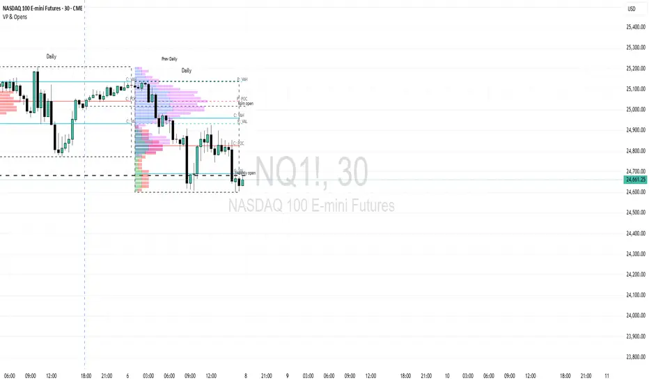
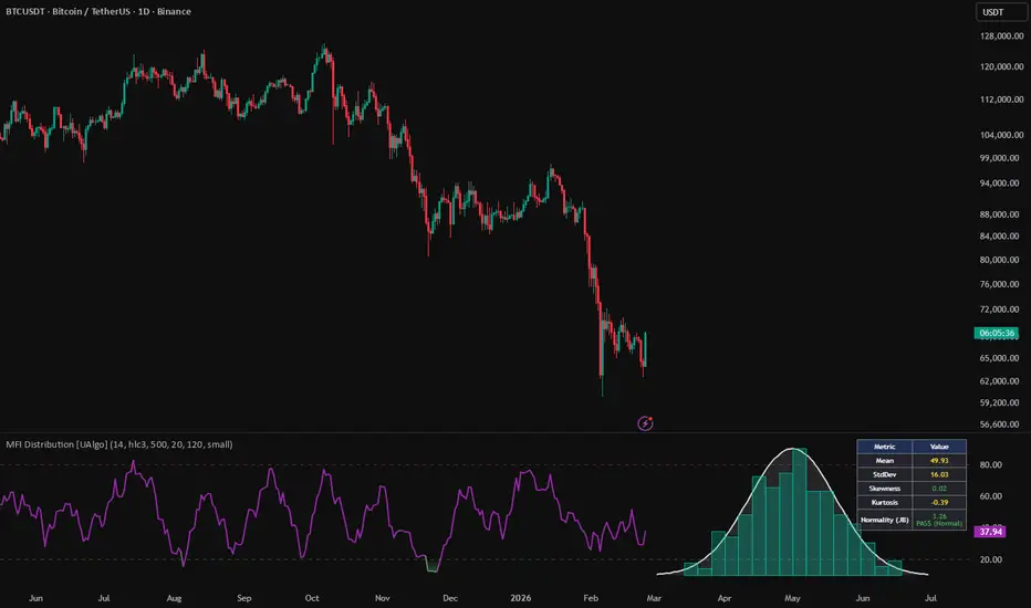
Sessions & VP with prev session VP & daily/weekly opensThis indicator combines two fully independent volume profile pipelines into a single overlay — one tracking the current session in real time, and one tracking the previous session — along with optional forex session boxes and daily/weekly open levels.
Both volume profiles are built from lower-timeframe intraday bar data (request.security_lower_tf), meaning each profile reflects the true distribution of volume across the session's price range rather than a single-bar approximation. The session range is divided into equal price bins, and each bin's volume is split into bullish and bearish components using a proportional wick/body weighting method. The Point of Control (POC), Value Area High (VAH), and Value Area Low (VAL) are calculated using standard Market Profile methodology.
The previous session VP is displayed as an overlay across the current session's bar range, making it easy to compare where the prior session's volume clustered against current price action without cluttering historical candles.
WHAT IT SHOWS
Current session: a live-updating volume profile drawn across the current session as it builds, with POC, VAH, VAL, and an optional session box.
Previous session overlay: the most recently completed session's volume profile, drawn across the current session's bar range. Levels are prefixed with "P:" to distinguish them from current session levels (prefixed "C:").
Forex session boxes: optional high/low range boxes for the Tokyo, London, and New York sessions. These show the range only — no volume profile is calculated for forex sessions.
Open levels: a 6 PM ET daily open line and a 6 PM Sunday weekly open line, both extending forward from the open price. These mark the start of the futures trading day and trading week respectively, which are commonly used reference levels in US equity index and futures trading.
HOW THE VOLUME PROFILE IS CALCULATED
Each session's price range (high to low) is divided into a user-defined number of equal bins. For every intraday bar within the session, volume is distributed across the bins it touches. Volume is further split into bullish (up-close) and bearish (down-close) by weighting the body and wick portions of each bar separately. This approach gives a more accurate picture of buyer and seller activity at each price level than simply assigning all of a bar's volume to a single bin.
The POC is the bin with the highest total volume. The Value Area expands outward from the POC, adding the next highest adjacent bin on either side, until cumulative volume reaches the user-defined percentage (default 70%).
Three display modes control how the histogram bars are rendered:
- Mode 1: bullish volume only, extending right from the session left edge
- Mode 2: bullish and bearish stacked left-to-right (standard side-by-side view)
- Mode 3: bullish extending right and bearish extending left from the session edge (mirrored)
SETTINGS
--- Current Session ---
Session Type — the period the current session covers. Options: Tokyo, London, New York, Daily, Weekly, Monthly, Quarterly, Yearly.
Show Volume Profile — toggle the histogram bars on/off.
Show POC — toggle the Point of Control line.
Show VAH and VAL — toggle the Value Area boundary lines.
Show Value Area Box — draws a filled rectangle covering the Value Area range.
Show Live Zone — when on, the current session profile updates in real time on every bar. When off, profiles are only drawn for completed sessions.
Show Session Box — draws a dashed outline box around the full session range.
Show Session Label — displays the session type name at the top of the session.
Resolution (default 30, min 5) — number of equal price bins. More bins gives finer detail. Note that each bin uses up to 2 boxes (one green, one red). With 30 bins and both current and previous sessions visible, up to 120 boxes are used, well within TradingView's 500-box limit.
Value Area % (default 70) — percentage of total session volume that defines the Value Area.
Bar Mode — controls the histogram layout. Mode 1 (bulls only), Mode 2 (side-by-side), Mode 3 (mirrored).
Profile Data — Volume uses standard bar volume. Open Interest uses the change in open interest (futures only).
Smooth Volume — applies a 5-period EMA to volume before building the profile.
--- Current Session Appearance ---
Up Volume color — fill color for bullish bins.
Down Volume color — fill color for bearish bins.
Value Area Box color — fill color for the Value Area Box if enabled.
POC, VAH, VAL — line color and thickness for each level.
Box — session box outline color and thickness.
--- Current Level Labels ---
Show Level Labels — toggles the POC/VAH/VAL text labels on/off.
POC Label, VAH Label, VAL Label — customise the text shown next to each level. Current session labels are prefixed "C:".
Label Size — tiny, small, normal, or large.
Label Text color.
--- Previous Session ---
All settings mirror the Current Session group above, with the following differences:
Show Overlay — when on, the previous session's volume profile is drawn across the current session's bar range. When off, no previous session profile is shown.
Previous session level labels are prefixed "P:" to distinguish them from current session levels.
--- Forex Sessions ---
Show Forex Session Boxes — when on, draws high/low range boxes for the Tokyo (midnight-9 UTC), London (7-16 UTC), and New York (13-22 UTC) sessions as each one closes. No volume profile is calculated for these — range only.
--- Open Levels ---
6 PM Daily Open — draws a horizontal line at the open price of the 6 PM ET bar, which marks the start of the US futures trading day. Line color, thickness, and style (solid, dotted, dashed) are configurable. Label toggle included.
Weekly Open (6 PM Sunday) — same as above but fires only on the Sunday 6 PM ET bar, marking the weekly futures open. Independently configurable color, thickness, style, and label.
IMPORTANT NOTES
- Best used on intraday timeframes (1m to 4H) so that lower-timeframe data is available to build accurate profiles. On daily or higher timeframes the profile will use only one bar per session and will be approximate.
- The previous session overlay requires at least two completed sessions of history before it appears.
- The current and previous session types are set independently and can be different (e.g. current = Daily, previous = Weekly).
- Open levels use America/New_York timezone regardless of chart timezone settings.
- Forex session boxes use UTC-based session detection. Results may vary on symbols with non-standard trading hours.
Credits: @LeviathanCapital for the excellent market sessions and volume profiles indicator on which this is based Wskaźnik

VP History WidgetVP History Widget plots a user-defined number of completed Volume Profiles (VPs) directly to the right of your price chart in real price coordinates. Each profile is calculated from the actual intraday bars that made up that session — giving an accurate picture of where volume was distributed across the price range of each past session. The sessions available are daily, weekly and monthly volume profiles.
Unlike volume profiles drawn on top of historical candles, this widget repositions all profiles into future bar space to the right of the current price, keeping your chart clean and uncluttered. Because everything is drawn in real price coordinates there is no distortion — profiles appear at exactly the correct size and price level relative to your chart.
HOW IT WORKS
Volume profiles are built using lower-timeframe intraday bar data (request.security_lower_tf), so the profile reflects the actual volume distribution across the session rather than a single-bar approximation. The session's price range is divided into a user-defined number of equal bins. For each bin, volume is split into bullish and bearish components using a proportional wick/body weighting method — the same approach used in professional volume profile tools. This data is stored in a rolling buffer and drawn on the last bar as a side-by-side histogram.
The Point of Control (POC) is the bin with the highest total volume. The Value Area High (VAH) and Value Area Low (VAL) are calculated by expanding outward from the POC until cumulative volume reaches the user-defined Value Area percentage (default 70%), following standard Market Profile methodology.
WHAT IT SHOWS
- Green histogram bars: volume from bullish (up-close) bars per price bin
- Red histogram bars: volume from bearish (down-close) bars per price bin
- POC line: price level with the highest volume for that session
- VAH / VAL lines: upper and lower boundaries of the Value Area
- Session labels: identify which session each profile belongs to (e.g. Daily -1, Daily -2)
TYPICAL USE CASES
- Identifying high-volume nodes (HVNs) and low-volume nodes (LVNs) from prior sessions as potential support and resistance
- Comparing volume distribution across multiple sessions to gauge market acceptance at price levels
- Spotting sessions where price moved quickly through a range — thin profiles indicate low acceptance and potential reversion zones
- Keeping your chart clean by comparing N previous session VPs without overlapping historical candles
SETTINGS
Show Widget — master on/off toggle.
Offset from price (default 10, range 1-50) — bars of space between the last candle and the first VP. Increase if profiles overlap your candles when zoomed out.
VP Width (default 10, range 3-40) — horizontal width of each volume profile in bars. Wider makes individual bins easier to read.
Gap between VPs (default 3, range 1-10) — spacing in bars between adjacent profiles.
Number of Sessions (default 5, range 1-10) — how many completed sessions to display. The most recent is on the right (marked with a triangle), oldest on the left.
Session Timeframe (Daily / Weekly / Monthly) — the period each volume profile covers.
VP Bins (default 50, range 5-50) — number of equal price buckets the session range is divided into. More bins gives finer resolution. With 5 sessions the maximum is 50 bins (5 x 50 x 2 = 500 boxes, TradingView's limit). With 10 sessions keep bins at 20 or below.
Value Area % (default 70, range 1-100) — percentage of total session volume that defines the Value Area. 70 is the standard Market Profile convention.
Profile Data (Volume / Open Interest) — Volume uses standard bar volume. Open Interest uses the change in OI, which requires a futures symbol with an OI feed.
Smooth Volume (default off) — applies a 5-period EMA to volume before building the profile, smoothing out single-bar spikes.
Up Volume color — fill color for bullish volume bins.
Down Volume color — fill color for bearish volume bins.
POC Line color — color of the Point of Control line.
VAH / VAL color — color of the Value Area boundary lines.
Separator color — color of the thin vertical line on the left edge of each VP slot.
Show POC — toggle the POC line and label on/off.
Show VAH / VAL — toggle Value Area boundary lines and labels on/off.
Show Labels — toggle all text labels on/off for a minimal look.
BOX LIMIT REFERENCE
TradingView limits indicators to 500 boxes. Each bin draws up to 2 boxes (green + red). Use this as a guide:
5 sessions — max 50 bins (500 boxes, at the limit)
6 sessions — max 40 bins (480 boxes)
7 sessions — max 35 bins (490 boxes)
8 sessions — max 30 bins (480 boxes)
9 sessions — max 27 bins (486 boxes)
10 sessions — max 24 bins (480 boxes)
If you see profiles with missing bars, reduce VP Bins or Number of Sessions.
IMPORTANT NOTES
- Best used on intraday chart timeframes (1m to 4H). When the chart timeframe equals the session timeframe, only a single candle is available and the profile will be approximate.
- The widget requires at least N+1 completed sessions of history to populate. On first load it may take a moment to build.
- Open Interest mode will silently fall back to volume on symbols without an OI feed. Wskaźnik

Liquidity Structure & Order Flow [UAlgo]Liquidity Structure & Order Flow is a range based market participation tool that combines a custom volume profile, value area analysis, liquidity void detection, and unusual volume tagging into a single chart overlay. Its goal is to show not only where volume has concentrated across price, but also how that activity was distributed between estimated buying pressure and selling pressure inside the recent market structure.
The script begins by scanning a rolling lookback range, then divides that vertical price space into a configurable number of bins. Each bin becomes a price segment that stores estimated buy volume, sell volume, and total volume. From there, the script builds a profile that highlights the Point of Control, the value area, and the internal order flow balance across the studied range.
What makes this indicator especially useful is that it does more than draw a standard profile. It also identifies areas where participation is abnormally thin relative to both the Point of Control and local neighboring bins. These low participation areas are marked as liquidity voids, helping the user see where the market moved through price with relatively little acceptance.
In addition, the script monitors the current bar for unusually large activity using a volume z score and a directional delta ratio filter. When a bar shows both exceptional size and meaningful directional imbalance, the script prints a bubble style marker above or below price. This gives the user a way to spot unusual participation events as they happen.
The result is a tool that can be used for profile analysis, liquidity mapping, imbalance recognition, and structural context. It helps answer several practical questions at once: where the market accepted price, where it rejected or skipped through price, where the strongest concentration of activity formed, and whether recent candles are showing exceptional directional participation.
🔹 Features
🔸 Custom Range Based Volume Profile
The script constructs a manual volume profile over the selected lookback period. Instead of relying on a built in profile engine, it divides the recent range into user defined price bins and allocates each bar’s volume into those bins. This gives full control over how the profile is built and how the final distribution is interpreted.
🔸 Buy Volume and Sell Volume Estimation
Every candle contributes both buy side and sell side estimates. The script uses the candle’s open, high, low, and close to derive a buy volume ratio, then splits total volume into buy volume and sell volume accordingly. This creates a practical order flow style approximation that is more informative than total volume alone.
🔸 Proportional Price Overlap Allocation
When a candle spans multiple bins, the script distributes its buy volume, sell volume, and total volume proportionally according to how much of the candle overlaps each bin. This produces a more realistic internal structure than simply dropping the full bar volume into one price row.
🔸 Point of Control Detection
The indicator finds the bin with the highest total volume and marks it as the Point of Control. This gives the user an immediate view of the strongest participation price inside the studied range.
🔸 Value Area Calculation
After the Point of Control is found, the script expands upward and downward through neighboring bins until the selected percentage of total profile volume is captured. This defines Value Area High and Value Area Low, allowing the user to distinguish the central acceptance region from the rest of the range.
🔸 Profile Coloring by Participation Side
The profile is drawn as stacked horizontal boxes showing estimated buy side participation and sell side participation inside each row. Bins inside the value area use stronger coloring, while bins outside the value area use softer coloring. This makes the internal structure easy to read visually.
🔸 Liquidity Void Detection
The script scans for bins with unusually weak participation outside the value area. A bin qualifies as a liquidity void candidate only if it is both small relative to the Point of Control and also weaker than its nearby neighbors. Consecutive weak bins are grouped into a larger void zone and labeled directly on the chart.
🔸 Unusual Volume Bubble Markers
Current bar activity is evaluated using a long period volume average and standard deviation. If the bar’s volume is statistically unusual and its estimated delta ratio is large enough, the script prints a directional bubble marker. Positive directional activity is shown below price, and negative directional activity is shown above price.
🔸 Optional Profile and Void Display
The user can independently control whether the volume profile, liquidity voids, and unusual volume markers are shown. This makes the script flexible enough for both full structure analysis and lighter chart layouts.
🔸 Extendable Structural Levels
The Point of Control, Value Area High, and Value Area Low can be drawn as either compact structure references or extended lines, depending on the chosen setting. This allows the user to decide whether the levels should function as local annotations or ongoing chart references.
🔸 Useful for Acceptance and Imbalance Analysis
The combination of profile structure, value area, void zones, and unusual activity markers gives the indicator a broader purpose than a standard profile. It can help identify accepted price, skipped price, directional participation, and possible future reaction areas.
🔹 Calculations
1) Building the Volume Profile Container
type PriceBin
float price
float buyVol = 0.0
float sellVol = 0.0
float totalVol = 0.0
type VolumeProfile
float highPrice = na
float lowPrice = na
float binSize = na
array bins
float pocPrice = na
float pocVol = 0.0
float vah = na
float val = na
float totalVol = 0.0
This is the foundation of the whole script.
Each PriceBin stores one price level area inside the profile. It contains:
the row midpoint price,
estimated buy volume,
estimated sell volume,
and total volume.
The VolumeProfile structure stores the full profile state:
the highest price of the lookback range,
the lowest price of the lookback range,
the bin size,
the array of bins,
and the final analytical values such as Point of Control, Value Area High, Value Area Low, and total profile volume.
So before any analysis happens, the script defines a complete custom data model for price distribution and order flow style estimation.
2) Initializing the Bins Across the Lookback Range
method initBins(VolumeProfile this, float h, float l, int numBins) =>
this.highPrice := h
this.lowPrice := l
this.binSize := (h - l) / numBins
this.pocPrice := na
this.pocVol := 0.0
this.totalVol := 0.0
this.vah := na
this.val := na
this.bins := array.new()
for i = 0 to numBins - 1
this.bins.push(PriceBin.new(price = l + i * this.binSize + (this.binSize / 2)))
This method creates the working profile rows.
First, it stores the high and low of the selected lookback period. Then it calculates binSize , which is the vertical price height of each row. That is simply the full range height divided by the number of bins.
After resetting all major profile outputs, the script creates a fresh bin array. Each new bin is assigned a midpoint price:
l + i * this.binSize + (this.binSize / 2)
That midpoint becomes the visual and analytical center of the row.
In practical terms, this is where the script transforms the raw market range into a structured ladder of price rows that can later receive allocated volume.
3) Locating the Correct Bin for a Price
method getBinIndex(VolumeProfile this, float p) =>
if na(this.lowPrice) or na(this.binSize) or this.binSize == 0
0
else
int idx = math.floor((p - this.lowPrice) / this.binSize)
math.max(0, math.min(idx, this.bins.size() - 1))
This helper method maps any price to its correct row index inside the profile.
It works by measuring how far the price sits above the profile low, then dividing that distance by the bin size. The result is the raw row index. After that, the value is clamped so it always stays inside the valid bin range.
This is important because the script repeatedly needs to know which rows are touched by each candle’s low and high. Without this mapping step, the profile could not distribute volume across price space correctly.
4) Estimating Buy Volume and Sell Volume From Candle Structure
float hlR = high - low
float bVR = hlR == 0 ? 0.5 : (close - low + high - open) / (2 * hlR)
float currentBuyVol = volume * bVR
float currentSellVol = volume * (1 - bVR)
float delta = currentBuyVol - currentSellVol
This snippet explains how the script approximates order flow direction on the current bar.
First, it measures the candle range from high to low. Then it computes a buy volume ratio using the relative location of the open and close inside that range:
(close - low + high - open) / (2 * hlR)
This ratio becomes a practical estimate of how much of the bar’s total volume behaved like buying pressure versus selling pressure. If the candle closes stronger and opens higher inside its range, the ratio leans more bullish. If the candle structure is weaker, the ratio leans more bearish.
That ratio is then used to split total volume into:
currentBuyVol
and
currentSellVol
Finally, the script calculates delta as the difference between estimated buy volume and estimated sell volume.
This is not true transaction tagged exchange delta, but it is a useful chart based directional participation model.
5) Distributing Candle Volume Across Touched Price Rows
method addBarVolume(VolumeProfile this, float h, float l, float c, float o, float v) =>
float hlRange = h - l
float buyVolRatio = hlRange == 0 ? 0.5 : (c - l + h - o) / (2 * hlRange)
float buyV = v * buyVolRatio
float sellV = v * (1 - buyVolRatio)
int startIdx = this.getBinIndex(l)
int endIdx = this.getBinIndex(h)
for i = startIdx to endIdx
if i >= 0 and i < this.bins.size()
PriceBin b = this.bins.get(i)
float binTop = b.price + (this.binSize / 2)
float binBot = b.price - (this.binSize / 2)
float overlapTop = math.min(h, binTop)
float overlapBot = math.max(l, binBot)
float overlap = math.max(0.0, overlapTop - overlapBot)
float weight = hlRange > 0 ? overlap / hlRange : (1.0 / (endIdx - startIdx + 1))
b.buyVol += buyV * weight
b.sellVol += sellV * weight
b.totalVol += v * weight
this.bins.set(i, b)
this.totalVol += v * weight
This is one of the most important calculations in the entire script.
For each candle inside the lookback period, the script first computes estimated buy volume and sell volume. Then it finds which profile rows are touched by the candle’s low and high.
For every touched row, it measures how much of the candle overlaps that specific row. That overlap becomes a weighting factor:
weight = overlap / hlRange
If a candle overlaps a row heavily, that row receives a larger share of the bar’s volume. If the overlap is small, the row receives only a small share.
The script then adds weighted buy volume, weighted sell volume, and weighted total volume into that bin.
This is much more realistic than assigning all volume to a single row because it respects the actual price space the candle traveled through.
6) Determining the Point of Control
method calcValueArea(VolumeProfile this, float pct) =>
float midPrice = (this.highPrice + this.lowPrice) / 2
float maxVol = -1.0
float bestPrice = na
int pocIdx = -1
for i = 0 to this.bins.size() - 1
PriceBin b = this.bins.get(i)
if b.totalVol > maxVol
maxVol := b.totalVol
bestPrice := b.price
pocIdx := i
else if b.totalVol == maxVol and maxVol > 0
if math.abs(b.price - midPrice) < math.abs(bestPrice - midPrice)
bestPrice := b.price
pocIdx := i
this.pocVol := maxVol
this.pocPrice := bestPrice
This is the first phase of the value area calculation.
The script scans all bins and finds the row with the greatest total volume. That row becomes the Point of Control. If two rows have the same maximum volume, the script breaks the tie by choosing the one closer to the middle of the full lookback range.
That tie handling matters because it avoids unstable selection when multiple bins have identical strength.
After the winning row is found, the script stores:
the Point of Control volume in pocVol
and the Point of Control price in pocPrice
So the Point of Control is not simply a visual midpoint. It is the actual strongest participation row in the profile.
7) Expanding Upward and Downward to Build the Value Area
float targetVol = this.totalVol * pct / 100.0
float currentVol = 0.0
if pocIdx >= 0 and pocIdx < this.bins.size()
currentVol := this.bins.get(pocIdx).totalVol
int upIdx = pocIdx + 1
int dnIdx = pocIdx - 1
while currentVol < targetVol and (upIdx < this.bins.size() or dnIdx >= 0)
float upVol = upIdx < this.bins.size() ? this.bins.get(upIdx).totalVol : -1.0
float dnVol = dnIdx >= 0 ? this.bins.get(dnIdx).totalVol : -1.0
After finding the Point of Control, the script calculates the target volume required for the value area. For example, if the input is 70 percent, the target becomes 70 percent of total profile volume.
The expansion begins from the Point of Control row itself. currentVol starts with the Point of Control row’s own total volume. Then the script looks one row up and one row down, repeatedly expanding until the accumulated volume reaches the target.
This is the standard logic of building a value area around the strongest participation center.
8) Deciding Whether to Expand Up or Down
if upVol > dnVol and upVol != -1.0
currentVol += upVol
upIdx += 1
else if dnVol > upVol and dnVol != -1.0
currentVol += dnVol
dnIdx -= 1
else if upVol == dnVol and upVol != -1.0
if currentVol + upVol > targetVol
if math.abs(this.bins.get(upIdx).price - midPrice) < math.abs(this.bins.get(dnIdx).price - midPrice)
currentVol += upVol
upIdx += 1
else
currentVol += dnVol
dnIdx -= 1
else
currentVol += upVol + dnVol
upIdx += 1
dnIdx -= 1
This block decides which side to include next in the value area.
If the row above has more volume than the row below, the script expands upward. If the row below has more volume, it expands downward. If both sides are equal, it uses distance to the overall midpoint as a tie breaker when necessary.
This is important because value area growth should follow participation strength, not arbitrary direction. The final result is a value area that naturally wraps around the highest volume concentration.
9) Final VAH and VAL Assignment
int finalUpIdx = math.max(pocIdx, upIdx - 1)
int finalDnIdx = math.min(pocIdx, dnIdx + 1)
this.vah := finalUpIdx < this.bins.size() ? this.bins.get(finalUpIdx).price : this.highPrice
this.val := finalDnIdx >= 0 ? this.bins.get(finalDnIdx).price : this.lowPrice
Once expansion is complete, the script converts the final included rows into value area boundaries.
The highest included row becomes Value Area High.
The lowest included row becomes Value Area Low.
These values define the central price zone where the chosen percentage of the profile’s total volume was traded.
So VAH and VAL are directly derived from the row by row structure of the profile, not from any fixed percentage of price range.
10) Detecting Unusual Volume Activity
float volSma = ta.sma(volume, 200)
float volStdev = ta.stdev(volume, 200)
float zScore = volStdev == 0 ? 0 : (volume - volSma) / volStdev
float deltaRatio = volume > 0 ? math.abs(delta) / volume : 0
bool isUnusual = zScore > zScoreThreshold and deltaRatio >= deltaRatioThreshold
This block evaluates whether the current bar is unusually active.
First, the script computes a 200 period average volume and standard deviation. Then it transforms the current bar’s volume into a z score, which shows how many standard deviations the bar stands above normal background activity.
Next, it calculates deltaRatio , which measures how large the directional imbalance is relative to total volume.
A bar is marked unusual only if both conditions are true:
the volume is statistically large enough,
and the directional imbalance is meaningful enough.
This double filter helps reduce false signals from large but directionless bars.
11) Printing Unusual Volume Bubbles
if showUnusual and isUnusual
string lblText = (delta > 0 ? "🟢 " : "🔴 ") + str.tostring(math.round(volume))
color lblColor = delta > 0 ? color.new(color.green, 0) : color.new(color.red, 0)
label uLbl = label.new(bar_index, delta > 0 ? low : high, text=lblText, style=label.style_none, textcolor=lblColor, yloc=delta > 0 ? yloc.belowbar : yloc.abovebar, size=size.small)
When an unusual bar is detected, the script prints a directional marker.
If estimated delta is positive, the bubble is shown below price in green.
If estimated delta is negative, the bubble is shown above price in red.
The displayed text also includes the rounded volume value. This allows the user to quickly see both direction and size of the unusual participation event.
So these markers are not random momentum tags. They specifically highlight bars where both participation size and directional imbalance stand out.
12) Rebuilding the Profile on the Last Bar
float highestPrice = ta.highest(high, lookback)
float lowestPrice = ta.lowest(low, lookback)
if barstate.islast and bar_index >= lookback - 1
profile.initBins(highestPrice, lowestPrice, rows)
for i = 0 to lookback - 1
profile.addBarVolume(high , low , close , open , volume )
profile.calcValueArea(vaPct)
This is the main execution block for the profile.
First, the script finds the highest high and lowest low across the chosen lookback window. That defines the total vertical space of the analysis.
Then, on the last visible bar, it:
initializes the bins,
loops through every candle inside the lookback,
adds each candle’s weighted volume into the profile,
and finally calculates the value area.
Running this only on the last bar is efficient because the full profile is a visual structure based on the current lookback window. It does not need to be redrawn historically on every past bar.
13) Scaling and Drawing the Profile Histogram
float maxVol = profile.pocVol
float allVols = array.new_float()
for i = 0 to profile.bins.size() - 1
allVols.push(profile.bins.get(i).totalVol)
float avgVol = allVols.avg()
float stdVol = allVols.stdev()
float clampedMaxVol = math.max(math.min(maxVol, avgVol + (stdVol * 2)), 0.000001)
Before drawing the profile, the script prepares a safer scaling reference.
Instead of using raw Point of Control volume alone without adjustment, it clamps the maximum drawable scale using the average row volume plus two standard deviations. This helps prevent a single extreme row from making the rest of the profile look too compressed.
In practical terms, this means the visual histogram remains readable even when one row is exceptionally dominant.
14) Drawing Buy Side and Sell Side Inside Each Row
int buyLen = math.round((b.buyVol / b.totalVol) * (drawVol / clampedMaxVol) * profileWidth)
int sellLen = math.round((b.sellVol / b.totalVol) * (drawVol / clampedMaxVol) * profileWidth)
bool inVA = b.price <= profile.vah and b.price >= profile.val
bool isPocRow = math.abs(b.price - profile.pocPrice) <= profile.binSize * 0.5
int x1 = profileRight
int x2 = x1 - buyLen
if buyLen > 0
box bB = box.new(x1, topP, x2, botP, border_color=c_border, bgcolor=c_buy)
int x3 = x2
int x4 = x3 - sellLen
if sellLen > 0
box bS = box.new(x3, topP, x4, botP, border_color=c_border, bgcolor=c_sell)
This is the actual profile drawing logic.
For each row, the script determines how much of the row’s total activity came from estimated buy volume and how much came from estimated sell volume. It then converts those fractions into horizontal lengths.
The buy portion is drawn first, then the sell portion continues from the end of the buy section. This creates a stacked horizontal bar that reveals both total participation and internal directional composition.
The row also receives context coloring:
rows inside the value area use stronger color treatment,
and the Point of Control row can receive a distinct border.
So the histogram communicates three layers at once:
how much volume was traded there,
whether that row sits inside the value area,
and how that row’s activity was split between estimated buying and selling pressure.
15) Drawing POC, VAH, and VAL Lines
line pocL = line.new(lineStartX, profile.pocPrice, lineEndX, profile.pocPrice, color=col_poc, width=2, style=line.style_solid)
profileLines.push(pocL)
line vahL = line.new(lineStartX, profile.vah, lineEndX, profile.vah, color=col_vah, width=1, style=line.style_dashed)
profileLines.push(vahL)
line valL = line.new(lineStartX, profile.val, lineEndX, profile.val, color=col_val, width=1, style=line.style_dashed)
profileLines.push(valL)
Once the profile is built, the script draws the three most important structural references:
Point of Control,
Value Area High,
and Value Area Low.
These lines can behave as compact annotations near the profile or as broader structure references if extension is enabled.
This gives the user a quick way to read acceptance and central balance without needing to inspect every row manually.
16) Detecting Liquidity Voids
float voidLimit = profile.pocVol * (voidThreshold / 100.0)
bool inVoid = false
float voidStartPrice = na
for i = 0 to profile.bins.size() - 1
PriceBin b = profile.bins.get(i)
bool isOutsideVA = b.price > profile.vah or b.price < profile.val
This is the beginning of the liquidity void logic.
A row is never treated as a void candidate solely because its volume is small. The script first requires that the row be outside the value area. This matters because low volume inside the main acceptance zone does not carry the same meaning as low volume outside it.
The script also calculates voidLimit as a percentage of Point of Control volume. That creates a relative participation threshold tied to the strongest row in the profile.
17) Comparing Each Row to Its Neighbors
float sumNeighbors = 0.0
int nC = 0
for j = math.max(0, i - 2) to math.min(profile.bins.size() - 1, i + 2)
if j != i
sumNeighbors += profile.bins.get(j).totalVol
nC += 1
float localAvg = nC > 0 ? sumNeighbors / nC : 0.0
bool isGap = b.totalVol < (localAvg * 0.5)
bool isLowVol = b.totalVol < voidLimit
bool isVoid = isLowVol and isGap and isOutsideVA
This is the real filter that defines a liquidity void.
The script looks at nearby bins around the current row and calculates a local neighbor average. Then it applies two separate tests:
the row must be low relative to the Point of Control threshold,
and it must also be weak relative to its nearby neighbors.
Only if both are true, and the row is outside the value area, does the script classify it as a void.
This is important because it prevents the indicator from marking every low volume row as a void. A valid void must look weak both globally and locally.
18) Grouping Consecutive Void Rows Into Zones
if isVoid
if not inVoid
inVoid := true
voidStartPrice := b.price - (profile.binSize / 2)
else
if inVoid
inVoid := false
float voidEndPrice = b.price - (profile.binSize / 2)
float topCoord = math.max(voidStartPrice, voidEndPrice)
float botCoord = math.min(voidStartPrice, voidEndPrice)
box vBox = box.new(bar_index - lookback, topCoord, bar_index, botCoord, border_color=na, bgcolor=col_void)
Once a void row is detected, the script begins tracking a continuous void run. If the next row is also a void, the zone continues. When the run ends, the script closes the zone and draws a box covering the full void area.
This means the indicator does not plot isolated tiny marks for each row. Instead, it groups neighboring weak rows into a cleaner structure that better represents a meaningful liquidity gap.
That box is then labeled as a liquidity void, making the zone easy to identify visually. Wskaźnik

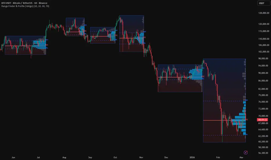
Range Finder & Profile [UAlgo]Range Finder & Profile is a structured market range detection tool that combines pivot based range discovery with an embedded volume profile. Its purpose is to identify areas where price begins to rotate inside a defined boundary, track whether that balance remains intact, and then summarize how volume was distributed inside the completed range once price finally exits it.
The script starts by using pivot highs and pivot lows to define potential horizontal boundaries. When a valid upper and lower reference exist, and price is trading inside those bounds without already breaking them, the script opens a candidate range. From that point onward, it keeps monitoring the structure bar by bar, checking whether the range survives long enough to become confirmed and whether price remains accepted inside it.
What makes this indicator especially useful is that it does not stop at simply drawing a box around consolidation. Once a range becomes confirmed, it also builds a row based internal profile of all activity inside that zone. When the range eventually breaks, the script calculates Point of Control, Value Area High, and Value Area Low, then draws a compact profile directly inside the range. This transforms a simple horizontal box into a more informative market acceptance map.
The result is a tool that can help traders study balance, distribution, and eventual expansion. It is useful for identifying clean consolidation structures, understanding where the heaviest participation occurred inside a range, and interpreting whether the breakout happened after meaningful internal acceptance or after a less developed structure.
🔹 Features
🔸 Pivot Based Range Discovery
The script uses pivot highs and pivot lows to establish potential range boundaries. This creates a structure that reacts to meaningful swing points rather than arbitrary rolling highs and lows. As a result, the detected ranges tend to reflect actual market rotation more naturally.
🔸 Clean Range Validation
A new range is only created when price is already trading inside the proposed top and bottom boundaries and when no bar in the candidate history has already closed outside those levels. This helps prevent invalid or already broken ranges from being accepted.
🔸 Overlap Protection
The script tracks where the last completed range ended and avoids creating a new one that starts inside an already closed structure. This reduces repeated overlap and keeps the chart cleaner.
🔸 Minimum Range Confirmation
Not every detected range is immediately treated as valid. The structure must survive for a minimum number of bars before it becomes confirmed. This helps filter out weak or short lived consolidations.
🔸 Embedded Volume Profile
Each confirmed range contains its own internal volume profile. The vertical height of the range is divided into configurable rows, and every bar contributes volume into the relevant price segments. This creates a compact distribution map inside the actual range boundaries.
🔸 Proportional Volume Allocation
The script does not simply drop full bar volume into a single row unless the bar has no height. Instead, when a candle spans multiple rows, its volume is distributed proportionally across the overlapped sections. This produces a more realistic representation of participation across the range.
🔸 Point of Control Detection
After the range is complete, the script finds the profile row with the highest accumulated volume. This row becomes the Point of Control, giving the user a quick view of the price area with the strongest concentration of activity.
🔸 Value Area Calculation
The script expands outward from the Point of Control and accumulates neighboring rows until the selected percentage of total range volume is reached. This produces Value Area High and Value Area Low, which highlight the area where most participation occurred.
🔸 Gradient Range Background
The active and completed range is drawn with a multi slice background gradient between the upper and lower colors. This improves readability and gives the zone a more polished visual structure.
🔸 Histogram Inside the Range
When a range is confirmed and completed, the script draws horizontal histogram bars inside the zone. Rows inside the value area use a dedicated color, while rows outside the value area use a separate profile color. This makes internal acceptance easy to read visually.
🔸 Live Active Range Updates
While the range is still active and not yet broken, the background extends forward in time with every new bar. Once the range becomes confirmed, profile and value area calculations are refreshed continuously until the breakout occurs.
🔸 Practical Market Structure Use
This makes the indicator useful for consolidation analysis, acceptance and rejection studies, and breakout context. A trader can see not only where price paused, but also how volume built inside that pause before expansion occurred.
🔹 Calculations
1) Pivot Detection for Range Anchors
float ph = ta.pivothigh(high, lengthInput, lengthInput)
float pl = ta.pivotlow(low, lengthInput, lengthInput)
if not na(ph)
recentPH := ph
recentPHIndex := bar_index
if not na(pl)
recentPL := pl
recentPLIndex := bar_index
This is the starting point of the whole script.
The code asks TradingView to detect a pivot high and a pivot low using the selected swing length. A pivot high appears only after enough bars have formed on both sides of the swing, and the same logic applies to a pivot low. Because of that, pivots are confirmed reference points rather than instant highs or lows.
When a valid pivot high is found, the script stores two things.
The pivot price itself in recentPH
The bar index where that pivot actually occurred in recentPHIndex
The same is done for pivot lows through recentPL and recentPLIndex .
This means the script always keeps track of the latest confirmed upper swing and the latest confirmed lower swing. Those two swing references become the raw ingredients for a possible trading range.
2) Candidate Range Creation Logic
bool canCreateRange = na(activeRange) and not na(recentPH) and not na(recentPL)
if canCreateRange
float top = math.max(recentPH, recentPL)
float bot = math.min(recentPH, recentPL)
if top > bot and close <= top and close >= bot
int sIndex = math.min(recentPHIndex, recentPLIndex)
int barsBack = bar_index - sIndex
This block decides whether the script is even allowed to start a new range.
First, canCreateRange requires three conditions:
there must be no currently active range,
there must be a recent pivot high,
and there must be a recent pivot low.
If those conditions are met, the script builds a provisional upper bound and lower bound using the greater and smaller of the two pivot prices. Then it checks whether current price is actually inside that proposed range. This is important because it prevents the script from creating a range that price has already escaped.
The code also finds sIndex , which is the earlier of the two pivot bar indices. That earlier point becomes the true starting location of the range. Then barsBack measures how many bars ago the range began.
So at this stage, the script has a full candidate structure:
an upper price,
a lower price,
and a starting point in time.
3) Overlap Prevention and Broken History Check
bool isOverlapping = false
if sIndex <= lastClosedRangeEndIndex
isOverlapping := true
if not isOverlapping
bool broken = false
if barsBack > 0
for i = 0 to barsBack
if close > top or close < bot
broken := true
break
This section filters out bad candidates before a range is created.
First, the script checks whether the proposed start index falls inside or before the end of the last completed range. If it does, the new candidate is marked as overlapping and rejected. This keeps the indicator from repeatedly generating new boxes on top of old structures.
Next, even if there is no overlap, the script scans every bar from the proposed start point up to the present. It checks whether any close moved above the top boundary or below the bottom boundary. If that happened, the candidate is marked as broken.
This is a very important quality filter. It means the script does not simply connect two pivots and call that a range. It also verifies that price actually stayed accepted inside those boundaries over the full candidate history.
4) Initializing the Range Object
activeRange := RangeData.new(
startIndex = sIndex,
startTime = time ,
endIndex = bar_index,
endTime = time,
topPrice = top,
bottomPrice = bot,
isActive = true,
isConfirmed = false,
totalVolume = 0.0,
pocPrice = na, pocVolume = 0.0, pocIndex = -1, vah = na, val = na,
bgBoxes = na, histBoxes = na, pocLine = na, vahLine = na, valLine = na, pocLabel = na, vahLabel = na, valLabel = na
)
activeRange.initProfile(profileRows)
Once the script is satisfied that the candidate is valid, it creates a new RangeData object.
This object stores all important information about the range:
where it starts,
where it currently ends,
its top price,
its bottom price,
whether it is still active,
whether it is confirmed,
and all profile related values such as total volume, Point of Control, Value Area High, and Value Area Low.
Immediately after creating the object, the script calls initProfile(profileRows) . That method prepares the internal volume profile rows that will later hold the distribution data.
So this is the moment where the script moves from pure detection into active tracking.
5) Building the Internal Profile Rows
method initProfile(RangeData this, int rowsCount) =>
float step = (this.topPrice - this.bottomPrice) / rowsCount
this.profile := array.new()
for i = 0 to rowsCount - 1
float pBottom = this.bottomPrice + (i * step)
float pTop = pBottom + step
this.profile.push(ProfileRow.new(pTop, pBottom, 0.0))
This method divides the height of the range into a fixed number of rows.
First, it calculates step , which is the height of one profile row. That is simply the total range height divided by the selected number of profile rows.
Then it creates an empty profile array and fills it row by row. Each row stores:
its upper price,
its lower price,
and the total volume accumulated in that row.
At this moment, every row starts with zero volume. The profile is just an empty framework waiting to receive bar by bar contributions.
This design is important because the script is not using a prebuilt TradingView volume profile function. It is constructing the profile manually, row by row, inside the exact range boundaries.
6) Adding Volume Into the Profile
method addVolume(RangeData this, float bHigh, float bLow, float bVol) =>
float overlapHigh = math.min(bHigh, this.topPrice)
float overlapLow = math.max(bLow, this.bottomPrice)
if bHigh == bLow and bHigh <= this.topPrice and bHigh >= this.bottomPrice
for i = 0 to this.profile.size() - 1
ProfileRow row = this.profile.get(i)
if bHigh >= row.priceBottom and bHigh <= row.priceTop
row.volumeTotal += bVol
this.totalVolume += bVol
break
else if overlapHigh > overlapLow
float overlapHeight = overlapHigh - overlapLow
float totalHeight = bHigh - bLow
float effectiveVol = totalHeight > 0 ? bVol * (overlapHeight / totalHeight) : bVol
for i = 0 to this.profile.size() - 1
ProfileRow row = this.profile.get(i)
float rowOverlapHigh = math.min(overlapHigh, row.priceTop)
float rowOverlapLow = math.max(overlapLow, row.priceBottom)
if rowOverlapHigh > rowOverlapLow
float rowOverlapHeight = rowOverlapHigh - rowOverlapLow
float rowRatio = rowOverlapHeight / overlapHeight
float addedVol = effectiveVol * rowRatio
row.volumeTotal += addedVol
this.totalVolume += addedVol
This is one of the most important calculations in the whole script.
The goal here is to take a candle and distribute its volume into the profile rows that the candle actually overlaps.
First, the script limits the candle to the range boundaries using overlapHigh and overlapLow . This ensures that only the part of the candle inside the range contributes to the profile.
Then two cases are handled.
If the candle has no height, meaning bHigh == bLow , the full volume is assigned to the single row that contains that exact price.
If the candle does have height, the script calculates how much of the candle actually overlaps the range. That overlapping height becomes the valid section for profile allocation. Then, for each profile row, the script measures how much of that valid section overlaps the row. Volume is distributed proportionally according to that overlap share.
This is much more accurate than placing the full candle volume into a single row. It means tall candles contribute volume across the price levels they truly passed through, which creates a more realistic internal distribution.
7) Filling the New Range With Historical Volume
if barsBack >= 0
for i = 0 to barsBack
float bVol = na(volume ) ? 1.0 : volume
activeRange.addVolume(high , low , bVol)
Right after a new range is created, the script goes back through all bars that belong to that range from its start until the current bar.
For each of those bars, it reads the volume and sends the bar high, bar low, and volume into addVolume .
This step is essential because it backfills the profile immediately. Without it, the range would start with an empty volume profile and would only accumulate data from future bars. Instead, the script reconstructs the whole internal history of the range as soon as the range is created.
Also notice the fallback 1.0 when volume data is missing. That ensures the script can still function on symbols where actual volume may not be available.
8) Range Confirmation and Break Detection
bool isBroken = close > activeRange.topPrice or close < activeRange.bottomPrice
if (bar_index - activeRange.startIndex) >= minRangeLen
activeRange.isConfirmed := true
Once a range is active, the script keeps evaluating two key questions on every bar.
The first question is whether the range is broken.
If the current close moves above the top or below the bottom, the range is considered finished.
The second question is whether the range has lasted long enough to be trusted.
If the number of bars since the range started is at least the user selected minimum, isConfirmed becomes true.
This creates a useful distinction between a candidate range and a confirmed range. A short structure can exist visually for a while, but it only becomes analytically meaningful after it survives long enough.
9) Live Updating While the Range Is Active
if not justCreated
float barVol = na(volume) ? 1.0 : volume
activeRange.addVolume(high, low, barVol)
if activeRange.isConfirmed
activeRange.calcValueArea(valAreaPct)
activeRange.drawProfile(colorBgTop, colorBgBot, colorProfile, colorProfileVA, colorPOC, colorVA)
else
activeRange.updateBgRight(time, colorBgTop, colorBgBot, colorBorder)
This block explains how the range evolves in real time.
If the current bar is not the same bar where the range was created, the script adds the latest candle volume into the profile. That keeps the internal distribution up to date bar by bar.
Then the script behaves differently depending on confirmation state.
If the range is already confirmed, it recalculates the value area and redraws the full profile. This means Point of Control, Value Area High, Value Area Low, and the histogram are all updated continuously as long as price remains inside the range.
If the range is not yet confirmed, the script only extends the background box to the current time. In other words, the market structure is still being monitored, but the full profile is not drawn until the range has proven itself.
10) Point of Control Discovery
float maxVol = -1.0
int pIndex = -1
for i = 0 to this.profile.size() - 1
ProfileRow row = this.profile.get(i)
if row.volumeTotal > maxVol
maxVol := row.volumeTotal
pIndex := i
this.pocIndex := pIndex
this.pocVolume := maxVol
ProfileRow pocRow = this.profile.get(pIndex)
this.pocPrice := (pocRow.priceTop + pocRow.priceBottom) / 2.0
This is the first phase inside the value area calculation.
The script scans every profile row and looks for the one with the largest accumulated volume. That row becomes the Point of Control row.
Once that row is found, the script stores:
the row index in pocIndex ,
the largest row volume in pocVolume ,
and the row midpoint price in pocPrice .
So the Point of Control is not guessed from the center of the range or from price action alone. It is derived directly from the heaviest profile row.
11) Expanding to Build the Value Area
float targetVol = this.totalVolume * (pct / 100.0)
float currentVol = maxVol
int upIndex = pIndex + 1
int downIndex = pIndex - 1
while currentVol < targetVol and (upIndex < this.profile.size() or downIndex >= 0)
float upVol = upIndex < this.profile.size() ? this.profile.get(upIndex).volumeTotal : -1.0
float downVol = downIndex >= 0 ? this.profile.get(downIndex).volumeTotal : -1.0
if upVol == -1.0 and downVol == -1.0
break
Here the script begins with the Point of Control row and tries to accumulate enough neighboring volume to reach the selected percentage of total range volume.
First, it calculates targetVol , which is the amount of total volume required for the value area. For example, if the input is 70 percent, the target is 70 percent of the full profile volume.
The process then starts from the Point of Control row. currentVol begins at the Point of Control volume itself. From there, the script looks one row up and one row down and keeps expanding until the target is reached or no more rows remain.
This is the classic logic of building a value area around the highest participation zone.
12) Choosing Whether to Expand Up or Down
bool addUp = false
if upVol > downVol
addUp := true
else if downVol > upVol
addUp := false
else
int distUp = upIndex - pIndex
int distDown = pIndex - downIndex
if distUp < distDown
addUp := true
else if distDown < distUp
addUp := false
else
addUp := true
This section decides which side should be added next to the value area.
If the row above the current zone has more volume than the row below, the script expands upward.
If the row below has more volume, it expands downward.
If both sides have the same volume, the script breaks the tie by comparing distance from the Point of Control. If distance is also equal, it defaults upward.
This matters because value area construction should not be arbitrary. It should expand toward the heaviest nearby participation first. That keeps the final value area centered around the most meaningful volume concentration.
13) Final VAH and VAL Calculation
int finalUp = math.min(upIndex - 1, this.profile.size() - 1)
int finalDown = math.max(downIndex + 1, 0)
this.vah := this.profile.get(finalUp).priceTop
this.val := this.profile.get(finalDown).priceBottom
After expansion is complete, the script converts the final upper and lower included rows into actual price boundaries.
vah becomes the top of the highest included row.
val becomes the bottom of the lowest included row.
These two values form the value area envelope, showing the price zone that contains the selected percentage of all volume traded inside the range.
So the final value area is not a fixed distance from Point of Control. It adapts to the actual row by row distribution.
14) Drawing the Gradient Range Background
method drawBg(RangeData this, color cBgTop, color cBgBot, color cBorder, int rTime) =>
if not na(this.bgBoxes)
for b in this.bgBoxes
b.delete()
this.bgBoxes := array.new()
int bgSlices = 10
float sliceStep = (this.topPrice - this.bottomPrice) / bgSlices
for i = 0 to bgSlices - 1
float bBot = this.bottomPrice + (i * sliceStep)
float bTop = bBot + sliceStep
this.bgBoxes.push(box.new(this.startTime, bTop, rTime, bBot, border_color=na, bgcolor=sliceCol, xloc=xloc.bar_time))
This method handles the visual background of the range.
Before drawing anything new, the script deletes previously drawn background boxes. Then it splits the range vertically into ten slices. Each slice receives an interpolated color between the selected bottom background color and top background color.
Finally, each slice is drawn as a time based box from the range start to the chosen right edge time.
The result is a smooth vertical color transition across the range body, which makes the zone easier to read and visually separates upper and lower sections.
15) Drawing the Histogram, POC, VAH, and VAL
if this.isConfirmed
float maxVol = this.pocVolume
if maxVol > 0
int rangeTimeWidth = math.max(rightTime - this.startTime, 1000)
int maxTimeWidth = math.round(rangeTimeWidth * 0.35)
for i = 0 to this.profile.size() - 1
ProfileRow row = this.profile.get(i)
if row.volumeTotal > 0
float widthRatio = row.volumeTotal / maxVol
int boxTimeWidth = math.round(maxTimeWidth * widthRatio)
int boxLeftTime = rightTime - boxTimeWidth
bool inVA = (row.priceTop <= this.vah and row.priceBottom >= this.val)
color finalHistCol = inVA ? histVaCol : histCol
this.histBoxes.push(box.new(boxLeftTime, t, rightTime, b, border_color=na, bgcolor=finalHistCol, xloc=xloc.bar_time))
this.pocLine := line.new(this.startTime, this.pocPrice, rightTime, this.pocPrice, color=pocCol, style=line.style_solid, width=2, xloc=xloc.bar_time)
this.vahLine := line.new(this.startTime, this.vah, rightTime, this.vah, color=vaCol, style=line.style_dashed, width=1, xloc=xloc.bar_time)
this.valLine := line.new(this.startTime, this.val, rightTime, this.val, color=vaCol, style=line.style_dashed, width=1, xloc=xloc.bar_time)
This is the drawing engine for the completed profile.
For each row with volume, the script calculates a width ratio relative to the Point of Control volume. Rows with more volume receive wider histogram boxes. Rows with less volume receive narrower boxes.
That width is converted into time space, so the histogram grows leftward from the right edge of the range. This creates a compact in range horizontal profile.
The script also checks whether each row lies inside the value area. If it does, the row uses the value area histogram color. If it does not, it uses the normal profile color. This makes the high participation area visually distinct.
Finally, the script draws three key lines across the full width of the range:
Point of Control,
Value Area High,
and Value Area Low.
These lines convert the internal profile data into easy to read structure references on the chart.
16) What Happens When the Range Breaks
if isBroken
activeRange.isActive := false
activeRange.endIndex := bar_index
activeRange.endTime := time
if not activeRange.isConfirmed
if not na(activeRange.bgBoxes)
for b in activeRange.bgBoxes
b.delete()
else
activeRange.calcValueArea(valAreaPct)
activeRange.drawProfile(colorBgTop, colorBgBot, colorProfile, colorProfileVA, colorPOC, colorVA)
lastClosedRangeEndIndex := bar_index
activeRange := na
This block defines the final lifecycle of a range.
When price closes outside the range boundaries, the active structure is terminated. The script records the ending bar and ending time, then checks whether the range had ever become confirmed.
If the range was never confirmed, its background is deleted and the structure is discarded. This prevents weak or short lived ranges from leaving unnecessary clutter.
If the range was confirmed, the script performs a final value area calculation and profile draw on the completed structure. It also stores the ending index so future ranges do not overlap with this one.
Then the active range is cleared from memory, which allows the script to start searching for the next valid structure. Wskaźnik

Liquidity Depth [UAlgo]Liquidity Depth is a price distribution and participation map designed to show where market activity has concentrated across a recent trading range. Instead of focusing only on candle by candle direction, the script builds a structured profile of how volume has been allocated across price levels inside a rolling lookback window. The result is a visual depth curve that helps identify areas where buyers or sellers may have shown stronger relative presence.
The indicator works by taking the highest and lowest prices inside the selected lookback, dividing that range into evenly spaced bins, and then assigning bar volume into those bins using one of two distribution models. This transforms raw volume into a spatial map of activity, allowing traders to see where liquidity has accumulated rather than simply when it appeared.
A central strength of the script is that it separates participation into buy side and sell side estimates using candle direction as a practical heuristic. Bullish candles contribute to the buy side profile and bearish candles contribute to the sell side profile. While this is not exchange level bid ask data, it creates a highly usable approximation of directional participation that is often more intuitive for chart based analysis.
The profile is drawn directly on the chart as a right side structure with smoothed depth curves, shaded fills, a Point of Control line, contextual range framing, and automatically detected strong liquidity pockets. This makes the tool especially useful for traders who want to study where activity is clustering, where resistance or support may be forming, and which parts of the recent range are attracting stronger participation.
Because the output is overlay based and visually compact, Liquidity Depth can be used in a wide variety of workflows. It can complement trend analysis, help frame pullback entries, identify acceptance and rejection zones, or simply provide a clearer understanding of where recent market interest has been strongest.
🔹 Features
🔸 Price Range Liquidity Mapping
The script scans a rolling lookback window, identifies the active price range, and divides that space into a configurable number of bins. Each bin becomes a small price segment where participation is accumulated. This produces a clear distribution style view of liquidity across the full recent range.
🔸 Two Distribution Modes
The indicator supports two ways of assigning volume into the profile.
Close Bin places the full bar volume into the single bin that contains the closing price. This creates a sharper and more concentrated structure that emphasizes where bars finished.
Wick Spread distributes the bar volume evenly across all bins touched by the candle from low to high. This produces a broader and more spatially balanced profile that better represents the full path of the bar through price.
These two modes give the user control over whether the profile should be more precise and concentrated or more inclusive and range aware.
🔸 Buy Side and Sell Side Separation
The script maintains separate depth values for buying and selling participation. Bullish candles add volume to the buy side and bearish candles add volume to the sell side. This creates two distinct distribution curves that help reveal whether the lower part of the range is showing stronger buying interest or whether the upper part is attracting stronger selling interest.
🔸 Smoothed Liquidity Curves
Instead of plotting raw bin values only, the script applies curve smoothing to the side distributions. This creates a cleaner, more readable shape that reduces visual noise and highlights the underlying structure of participation. The result is a profile that feels fluid and analytical rather than fragmented.
🔸 Glow Enhanced Curve Rendering
The current build uses a glow style rendering around the main liquidity curves. This improves visual separation on the chart and makes strong participation bulges easier to recognize at a glance, especially when the profile is viewed on darker chart themes.
🔸 Automatic Strong Pocket Detection
One of the most practical parts of the script is its ability to detect strong liquidity pockets. These are clusters of consecutive bins where smoothed participation exceeds a chosen strength threshold. When found, the script highlights the zone and labels it as a strong buy pocket or strong sell pocket. These pockets can be useful for identifying areas of acceptance, defense, or possible future reaction.
🔸 Point of Control Highlighting
The indicator finds the price bin with the highest total participation and marks it as the Point of Control. This is the most active price area inside the profile and often serves as an important reference for equilibrium, attraction, or repeated interaction.
🔸 Range Frame and Midpoint Context
A visual frame is drawn around the active profile range, including the highest level, the lowest level, and the midpoint. This gives the distribution a clear structure and helps the user understand where participation is concentrated relative to the center of the recent range.
🔸 Side Summary Readout
The script prints a compact summary that shows estimated buy side and sell side percentages, along with total side volumes. This provides a quick interpretation layer so the user can understand the current balance of participation without needing to inspect each curve manually.
🔸 Theme Adaptive Colors
Colors are selected dynamically according to the chart background tone. This helps the profile remain readable across both light and dark themes while preserving clear differentiation between buy side, sell side, frame lines, and Point of Control.
🔸 Efficient Object Management
All boxes, lines, fills, and labels are refreshed on the last visible bar so the profile stays clean and up to date. Internal object arrays are actively cleared and rebuilt, which keeps the display organized and avoids uncontrolled accumulation of chart objects.
🔹 Calculations
1) Active Range Construction
The script begins by defining the working range from the highest high and lowest low across the selected lookback window. This creates the vertical space where the full profile will be built.
The total span is then divided into the configured number of bins, which creates evenly spaced price segments from the bottom of the range to the top. Each bin stores its lower boundary, upper boundary, midpoint, buy volume, sell volume, and total volume.
In practical terms, this means the indicator converts the recent market range into a structured ladder of price levels so activity can be measured spatially.
2) Bin Initialization
Once the range is known, every bin is reset and rebuilt. Each bin receives:
its lower boundary,
its upper boundary,
its midpoint,
and empty participation values for buy, sell, and total activity.
This reset process ensures that the profile always reflects only the current rolling window rather than carrying stale values from older bars.
3) Volume Assignment Logic
For every bar inside the lookback, the script reads the volume and determines whether the candle is bullish or bearish. From there, distribution depends on the selected mode.
With Close Bin , the full bar volume is assigned to the bin that contains the close. If the candle is bullish, that volume is counted on the buy side. If the candle is bearish, it is counted on the sell side.
With Wick Spread , the script finds every bin touched between the candle low and candle high. The bar volume is divided evenly across those crossed bins. That distributed share is then assigned entirely to the buy side for bullish candles or entirely to the sell side for bearish candles.
This approach creates a practical estimate of where participation occurred across price, while also preserving directional context.
4) Total Participation and Point of Control
After all bars are processed, each bin contains a buy volume, a sell volume, and a total volume equal to the sum of the two. The script then scans the full array of bins to find the highest total value. The bin with that maximum total becomes the Point of Control.
The Point of Control represents the most concentrated participation zone inside the profile and is drawn as a dedicated horizontal reference line.
5) Midpoint Split and Side Totals
The active range midpoint is calculated as the average of the range high and range low. This midpoint is used as the divider between the lower half and upper half of the profile.
For summary purposes, buy side totals are accumulated from bins at or below the midpoint, while sell side totals are accumulated from bins above the midpoint. The script also records the highest buy side bin value and the highest sell side bin value.
This design gives the profile a simple structural interpretation:
lower range strength is associated with buying participation,
upper range strength is associated with selling participation.
That makes the summary especially useful for understanding whether the range is showing stronger support style accumulation below or stronger supply style pressure above.
6) Smoothing Engine
To reduce jaggedness, the script smooths each side of the profile with a local weighted kernel built from five neighboring bins. The center bin carries the highest influence, adjacent bins carry moderate influence, and outer bins carry smaller influence.
The smoothed result is then blended with the raw bin value according to the user selected smoothing factor. A low smoothing value preserves more of the original structure, while a high smoothing value creates a softer and more continuous curve.
This process helps reveal the true shape of participation without overreacting to isolated bin spikes.
7) Curve Projection and Shape Refinement
Once a side is smoothed, its value is normalized against the maximum strength of that side. The normalized result is converted into horizontal width inside the selected profile width. This is what determines how far the curve extends to the right from its anchor point.
The script also applies an additional running refinement to the horizontal curve position from one bin to the next. This makes the drawn path more fluid and helps eliminate abrupt lateral jumps between neighboring levels.
The final effect is a polished depth curve that communicates intensity clearly while remaining visually smooth.
8) Strong Pocket Detection
Strong liquidity pockets are found by scanning for consecutive bins where normalized smoothed participation exceeds the pocket threshold.
For the upper half of the profile, the script searches for strong sell side runs.
For the lower half of the profile, the script searches for strong buy side runs.
When a qualifying run lasts for at least the minimum required number of bins, a zone is drawn across that price region and labeled accordingly. The horizontal size of the zone is linked to the peak strength found inside that run.
This means the pocket logic is not simply marking a single peak. It is identifying sustained participation clusters, which often carry more analytical value than isolated extremes.
9) Visual Frame and Range Guides
The script adds a top guide at the range high, a bottom guide at the range low, and a midpoint guide through the center of the profile. These references help the user interpret the shape of liquidity in relation to the broader active range.
A curve concentrated near the midpoint suggests balance or repeated acceptance.
A strong bulge in the upper section can imply stronger supply style participation.
A strong bulge in the lower section can imply stronger demand style participation.
10) Summary Metrics
The summary label presents estimated buy side and sell side percentages along with total side volumes. These percentages are derived from the midpoint based side totals described above.
This gives the user a fast read on the internal balance of the profile without needing to inspect the full shape manually. It is especially useful when comparing one instrument or one session structure to another. Wskaźnik
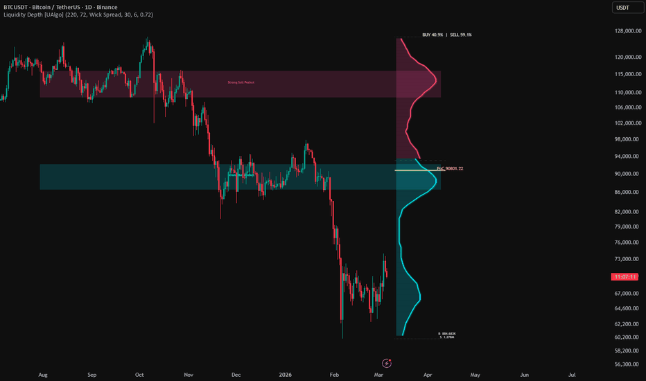
Delta Flow Volume Profile [UAlgo]Delta Flow Volume Profile is a price based profile indicator that builds a rolling volume distribution and separates that distribution into bullish and bearish participation at each price zone. Instead of showing only how much total volume traded in an area, the script splits each profile row into buyer dominated and seller dominated segments, then renders those segments side by side on the chart. This creates a more informative profile that helps reveal not only where activity concentrated, but also which side was dominant inside each level.
The indicator runs directly on price ( overlay=true ) and analyzes a user defined lookback window. It divides the recent price range into fixed bins, distributes each candle’s volume across the bins it overlaps, and classifies that allocated volume as bullish or bearish based on candle direction. The final result is drawn to the right of the chart as a horizontal stacked profile where:
The left segment of each row represents bullish volume
The right segment represents bearish volume
The widest total row identifies the Point of Control (POC)
Each significant row can display buyer and seller percentage labels
This makes the script useful for traders who want a profile style map of participation with directional context, especially when identifying areas where buyers were dominant, sellers were dominant, or both sides were highly active.
Important note: The bullish and bearish split in this script is an approximation based on candle direction ( close >= open versus close < open ). It is not true bid ask or tick level order flow delta.
🔹 Features
🔸 1) Delta Style Volume Profile by Price Level
The core idea of the script is to turn a standard horizontal volume profile into a directional participation profile. Each row tracks both bullish and bearish volume, so the user can see whether a price zone was primarily buyer controlled, seller controlled, or relatively balanced.
🔸 2) Rolling Lookback Profile
The profile is built from the most recent user selected number of bars. This means the profile continuously adapts to current market structure instead of being locked to a session boundary.
This makes it useful for intraday structure analysis, local range mapping, and recent participation studies.
🔸 3) Fixed Bin Price Segmentation
The script divides the recent highest to lowest range into a configurable number of bins. Lower bin counts create thicker and smoother rows. Higher bin counts create more detailed and granular distribution.
This lets the user control the balance between clarity and resolution.
🔸 4) Proportional Volume Allocation Across Overlapping Bins
When a candle spans multiple bins, the script does not place the full candle volume into a single row. Instead, it allocates volume proportionally according to the overlap between the candle range and each bin.
This produces a more realistic distribution than a single point assignment, especially for larger candles.
🔸 5) Bullish and Bearish Segment Rendering
Each row is drawn as a stacked two part structure:
The bullish segment starts from the left base of the profile
The bearish segment continues immediately after the bullish segment
This gives an intuitive visual read of which side dominated and how much each side contributed inside the same price zone.
🔸 6) Point of Control Highlighting
The script automatically finds the row with the highest total volume and marks it as the Point of Control. The POC row is highlighted with a full width background band, which makes the most active zone immediately obvious.
This is useful for identifying the strongest recent area of price acceptance.
🔸 7) Percentage Labels for Strong Rows
For profile rows with meaningful participation, the script prints a right side label showing:
Bullish percentage
Bearish percentage
For the POC row, the label is prefixed with POC . This gives a quick summary of directional balance at the most important nodes.
🔸 8) Dynamic Label Coloring by Dominance
The percentage labels change color based on row context:
POC labels use the dedicated POC color
Rows dominated by bullish volume use the bullish color
Rows dominated by bearish volume use the bearish color
This improves readability and speeds up visual interpretation.
🔸 9) Adjustable Profile Width and Offset
The profile is drawn to the right of the current bar with configurable:
Profile width as a percentage of lookback
Horizontal offset in bars
This makes it easy to place the profile in a clean position without obstructing live price action.
🔸 10) Smooth Clean Presentation
The script uses borderless boxes and compact right side labels, which gives the profile a clean and uncluttered look. This makes it suitable for traders who want visual structure without excessive chart noise.
🔸 11) Built for Practical Delta Style Context
While it does not use true order flow data, the indicator still provides a highly usable approximation of directional participation. This can help identify:
Buyer heavy zones
Seller heavy zones
Balanced zones
High activity acceptance areas
🔹 Calculations
1) Price Range Detection
The script first determines the highest high and lowest low over the selected lookback:
float hh_global = ta.highest(high, lookback)
float ll_global = ta.lowest(low, lookback)
This defines the full vertical range of the profile.
2) Bin Construction
That range is divided into the selected number of bins:
float binSize = (hh - ll) / numBins
Each bin stores:
Top price
Bottom price
Bullish allocated volume
Bearish allocated volume
The bins are built from top to bottom so the profile rows map naturally across the recent range.
3) Candle by Candle Volume Processing
For every bar in the lookback window, the script reads:
High
Low
Open
Close
Volume
Then it checks each bin to see whether the candle overlaps that bin.
4) Proportional Overlap Allocation
For each overlapping bin, the script calculates:
float overlapTop = math.min(bHigh, b.top)
float overlapBottom = math.max(bLow, b.bottom)
If there is overlap, it allocates volume proportionally:
allocatedVol := bVol * ((overlapTop - overlapBottom) / rangeSize)
Interpretation:
If a candle covers multiple price rows, each row receives only the fraction of volume corresponding to its share of the candle’s total range.
This is a more realistic approximation than assigning all volume to one bin.
5) Zero Range Candle Handling
If a candle has zero range, the script assigns the full volume to the bin that contains the candle price:
if rangeSize > 0
...
else
if bHigh <= b.top and (bHigh > b.bottom or (j == numBins - 1 and bHigh >= b.bottom))
allocatedVol := bVol
This prevents divide by zero issues and still keeps the data usable.
6) Bullish vs Bearish Classification
Once the script calculates allocated volume for a bin, it classifies that volume by candle direction:
if bClose >= bOpen
b.bullVol += allocatedVol
else
b.bearVol += allocatedVol
Interpretation:
Bullish volume means the candle closed at or above its open.
Bearish volume means the candle closed below its open.
Important note:
This is a directional approximation. It is not true tape based aggressive buy or aggressive sell volume.
7) Total Volume, Delta, and Percent Methods
Each bin includes helper methods:
totalVol() returns bullVol + bearVol
deltaVol() returns bullVol - bearVol
bullPct() returns bullish percentage of total
bearPct() returns bearish percentage of total
The script actively uses total volume and percentages in rendering. The deltaVol() method is defined for convenience, but this version does not directly plot or label the raw delta value.
8) Point of Control Detection
After all bins are populated, the script finds the row with the largest total volume:
if bTotVol > maxVol
maxVol := bTotVol
pocIdx := i
This row becomes the Point of Control and acts as the strongest recent participation zone.
9) Width Normalization
The total maximum row volume is used as the width normalization anchor. For each row:
float bullRatio = b.bullVol / maxVol
float bearRatio = b.bearVol / maxVol
Then the segment widths are scaled into bars:
int bullWidthBars = math.round(bullRatio * maxBoxWidthBars)
int bearWidthBars = math.round(bearRatio * maxBoxWidthBars)
Because both bullish and bearish widths are normalized against the same maxVol , their combined width reflects the row’s total participation relative to the profile maximum.
10) Minimum Visible Width Safeguard
If a row has non zero bullish or bearish volume but the calculated width rounds to zero, the script forces a minimum width of one bar:
if b.bullVol > 0 and bullWidthBars == 0
bullWidthBars := 1
This ensures small but meaningful contributions remain visible.
11) Right Side Time Based Layout
The profile is rendered using xloc.bar_time , so all horizontal distances are based on time, not bar index. The script calculates:
A base left time for the profile
A maximum right time
A per bar time width
Key logic:
int leftBaseTime = lastBarTime + (profileOffset * barTimeDiff)
int maxRightTime = leftBaseTime + (maxBoxWidthBars * barTimeDiff)
This makes the profile appear a fixed number of bar widths to the right of the latest candle.
12) POC Background Highlight
Before drawing the bullish and bearish segments for the POC row, the script paints a full width background band:
box.new(left=leftBaseTime, top=drawTop, right=maxRightTime, bottom=drawBottom, ...)
This gives the POC a distinct highlighted backdrop behind the actual stacked volume bars.
13) Visual Gap Inside Each Bin
The script trims the top and bottom of each drawn row slightly:
float boxGap = (b.top - b.bottom) * 0.1
float drawTop = b.top - boxGap
float drawBottom = b.bottom + boxGap
This creates small vertical spacing between rows, which improves readability and avoids a fully merged block appearance.
14) Percentage Label Threshold
Labels are not printed for every row. They appear only when the row’s total volume is greater than 15 percent of the maximum row volume:
if bTotVol > (maxVol * 0.15)
This reduces clutter and focuses attention on more relevant nodes.
15) Label Text Construction
For significant rows, the script computes:
Bullish percentage
Bearish percentage
Then formats them as:
string labelText = bullStr + " | " + bearStr
For the POC row:
labelText := "POC: " + labelText
Wskaźnik

Swing Profile [BigBeluga]🔵 OVERVIEW
Swing Profile is a dynamic swing-based volume profiling tool that builds a complete volume profile for each completed market swing.
Instead of using fixed sessions or time ranges, the indicator anchors its profile strictly between confirmed swing highs and swing lows, allowing traders to analyze where volume accumulated inside each directional leg.
The profile updates in real time while a swing is still forming and finalizes once the swing direction flips, giving both historical and live insight into volume behavior.
🔵 CONCEPTS
Swing-Anchored Profiling — Volume is calculated only between confirmed swing highs and lows detected by the Swing Length input.
Directional Legs — Each bullish or bearish swing leg gets its own independent volume profile.
ATR-Adaptive Bins — Profile bin size is automatically scaled using ATR, keeping resolution consistent across volatility regimes.
Real-Time Rebuild — While a swing is still active, the profile continuously recalculates and redraws.
Finalized Profiles — Once direction flips, the profile is locked and marked as a completed swing.
🔵 FEATURES
Swing Volume Profile — Displays horizontal volume distribution for each swing leg.
Point of Control (PoC) — Highlights the price level with the highest traded volume inside the swing.
Buy / Sell Volume Separation — Tracks bullish (buy) and bearish (sell) volume inside each profile.
Delta Volume Calculation — Shows net buying vs selling pressure as a percentage.
Profile Outline — A polyline traces the outer shape of the volume distribution.
HeatMap Mode — Optional heatmap visualization showing volume intensity by color gradient.
ZigZag Swing Connector — Visual connection between swing highs and lows for structure clarity.
Custom Label Sizing — Adjust label size (Tiny → Huge) for clean chart scaling.
🔵 HOW TO USE
Identify High-Interest Zones — Use the PoC to locate price levels where the market spent the most time during a swing.
Trend Strength Analysis — Strong directional swings often show volume skewed toward one side of the profile.
Pullback Zones — Profiles help identify areas where price may react during retracements.
Continuation vs Reversal — Delta volume reveals whether buying or selling dominated the swing.
Live Monitoring — While a swing is forming, watch the real-time profile to anticipate where structure may complete.
🔵 DATA LABELS
T — Total traded volume inside the swing.
B — Buy volume (bullish candles).
S — Sell volume (bearish candles).
D — Delta volume (% difference between buy and sell volume).
🔵 CONCLUSION
Swing Profile delivers a precise, structure-aware view of volume by anchoring profiles directly to market swings.
By combining real-time profiling, PoC detection, delta analysis, and adaptive resolution, it provides deep insight into where participation truly occurred — making it a powerful tool for swing traders, structure traders, and volume-focused strategies. Wskaźnik

3D Volume Profile [UAlgo]3D Volume Profile is a chart based volume profile indicator that takes a classic horizontal profile concept and presents it as a pseudo 3D structure directly on price. Instead of drawing flat histogram bars only, the script renders each profile row as a shaded 3D block with a front face, a side face, and a top face, which creates a stronger visual sense of depth and distribution.
The indicator runs on price ( overlay=true ) and builds a rolling volume profile over a user defined lookback window. It divides the recent price range into fixed bins, distributes candle volume across those bins, identifies the Point of Control and the Value Area, and then draws the result on the right side of the chart. Each row is color coded by dominant flow direction, which means the profile can show whether a bin was more buy dominated or sell dominated in addition to showing how much total volume accumulated there.
This makes the tool useful for traders who want more than a basic profile display. It combines:
A rolling horizontal volume profile
Buy versus sell dominance shading
Point of Control and Value Area detection
A forward projected 3D style histogram
Clear POC, VAH, and VAL reference lines on the chart
The final result is a visually rich profile tool designed for fast structural reading, especially when identifying acceptance zones, thin areas, and dominant participation regions.
🔹 Features
🔸 1) Rolling Volume Profile Over a Recent Window
The script builds a rolling profile from the most recent user selected number of bars. This means the profile continuously adapts as new bars come in, making it more useful for current market structure analysis than a fixed session only approach.
🔸 2) 3D Style Histogram Rendering
Each volume row is drawn as a pseudo 3D block rather than a flat rectangle. The script creates:
A front face
A side face
A top face
The side and top faces are shaded versions of the main color, which gives the profile a depth effect and makes the structure easier to read visually.
🔸 3) Customizable 3D Depth in X and Y
The 3D effect is controlled with two settings:
3D Depth X , which controls how far the rear face is shifted horizontally in bars
3D Depth Y , which controls how far the rear face is shifted vertically as a percentage of row height
This allows the user to make the profile look flatter or more pronounced depending on preference.
🔸 4) Buy and Sell Volume Dominance Coloring
Each bin tracks both buy volume and sell volume. If buy volume is greater than or equal to sell volume, the row uses the bullish color. If sell volume dominates, the row uses the bearish color.
This means the profile is not only a measure of total activity. It also adds directional context to each price zone.
🔸 5) Point of Control Detection
The script identifies the row with the highest total volume and marks it as the Point of Control. The POC is highlighted with its own dedicated color and is visually distinct from the rest of the profile.
This gives traders an immediate reference for the most active price zone in the rolling range.
🔸 6) Value Area Calculation
The indicator calculates a Value Area around the Point of Control based on the user selected percentage. Bins inside the Value Area are marked and recolored with the Value Area color, which makes the high participation region easy to identify.
🔸 7) Forward Projected Profile Layout
The profile is drawn to the right of current price using a configurable offset. This keeps the active candle area readable while still placing the profile in a clear and accessible location.
🔸 8) Adjustable Resolution and Width
Users can control:
The lookback length
The number of profile rows
The maximum width of the histogram
The right side offset
This makes the indicator suitable for both coarse structural analysis and more detailed profile inspection.
🔸 9) POC, VAH, and VAL Reference Lines
After the profile is built, the script calculates the POC, Value Area High, and Value Area Low, then projects horizontal reference lines across the chart. Labels are placed to the right so the key levels are clearly marked.
🔸 10) Row by Row Dominance and Acceptance Reading
Because each row stores total volume, buy volume, sell volume, Value Area membership, and POC status, the indicator gives a layered view of the market:
Where the most activity occurred
Which zones were accepted
Which zones were dominated by buyers
Which zones were dominated by sellers
🔸 11) Premium Visual Presentation
The script uses shaded faces, dedicated POC highlighting, Value Area recoloring, and clean right side labels. This makes it more presentation focused than a basic flat profile and improves chart readability for manual analysis.
🔹 Calculations
1) Profile Range Detection
The script first finds the highest high and lowest low inside the active lookback window. This defines the full vertical range of the volume profile. Only the most recent bars inside that window are used for profile construction.
2) Bin Initialization
Once the recent range is known, the script divides that price range into the chosen number of bins. Each bin stores:
Top boundary
Bottom boundary
Total volume
Buy volume
Sell volume
Flags for Value Area and POC
The bin size is calculated by dividing the total price range by the number of rows.
3) Volume Distribution Across Price Bins
For each candle, the script determines which bins the candle spans. It then spreads that candle’s volume evenly across all touched bins.
This is important because the script does not place the full candle volume into a single price level. Instead, it allocates the candle volume across the portion of the profile that candle covers.
Important implementation note:
This script uses equal distribution across the spanned bins, not proportional overlap weighting. That means each touched row receives the same share of the candle’s volume.
4) Buy Versus Sell Volume Classification
The script classifies each candle as buy dominated or sell dominated using candle direction:
If close is greater than or equal to open, the candle is treated as buy volume
If close is below open, the candle is treated as sell volume
That candle’s allocated volume is then added to either volBuy or volSell inside each touched bin.
This is a practical directional approximation, not true bid ask tape volume.
5) Total Volume and POC Detection
After all candles are processed, the script scans every bin and calculates:
The total volume across the profile
The maximum single bin volume
The POC index
The POC is the bin with the highest total volume. That bin is marked as both isPOC and isVA before Value Area expansion begins.
6) Value Area Expansion Logic
The Value Area is built around the POC by expanding upward and downward until the selected percentage of total profile volume is included.
The script compares the next bin above and the next bin below the current Value Area. It adds whichever side has greater volume first. This continues until cumulative included volume reaches the target Value Area percentage.
This creates a standard profile style Value Area centered on the highest participation region.
7) Histogram Width Normalization
Each row’s width is scaled relative to the maximum volume row:
The row with the most volume becomes the widest
Smaller rows are scaled proportionally
This means width directly communicates relative participation at each price zone.
8) Color Selection Logic
For each bin, the script first determines whether buy volume or sell volume dominates:
If buy volume is greater than or equal to sell volume, it uses the bullish color
Otherwise it uses the bearish color
Then the script overrides that base direction color if needed:
If the row is the POC, it uses the POC color
If the row is inside the Value Area, it uses the Value Area color
This gives the profile a clear visual hierarchy:
POC first
Value Area second
Directional dominance otherwise
9) 3D Face Construction
Each row is rendered as a pseudo 3D object using:
A front rectangle
A shifted back edge using the X and Y depth settings
A side face when horizontal depth is visible
A top or bottom face depending on vertical depth direction
The script shades the side face darker and the top face brighter than the base color to create a depth illusion.
This is a visual projection technique, not a true 3D engine, but it produces a convincing 3D profile effect on the chart.
10) Rendering Order Logic
The script changes draw order depending on the sign of the Y depth:
If vertical depth is positive, rows are drawn from bottom to top
If vertical depth is negative, rows are drawn from top to bottom
This helps the 3D faces stack more cleanly and reduces visual overlap issues.
11) POC, VAH, and VAL Price Calculation
After the profile is complete:
The POC price is the midpoint of the POC bin
VAH is the highest top boundary among all Value Area bins
VAL is the lowest bottom boundary among all Value Area bins
These levels are then drawn as horizontal lines extending from the left side of the lookback window toward the right side label area.
12) Label Placement
The labels for POC, VAH, and VAL are placed slightly to the right of the profile. This keeps them readable and avoids overlap with the 3D bars themselves. Wskaźnik

Value Area Levels [crlmx]Calculated from native volume-at-price data vaLevels shows Value Area
levels (VAH, POC, VAL) across three independently configurable timeframes.
Requires TradingView Premium or above plan for Footprint data access,
Short of that refere to Lite version (coming soon).
Key Features
- Three independent VA slots with on/off toggles
- Timeframe selection: D, W, M, 30min, 1H, 4H, 8H, 12H
- Session-based VA on slot 3: NYC, London, Asia, Custom
- Custom session with user-defined time window and label prefix
- Auto-calculated row resolution per instrument type
- Manual ticks-per-row override for fine-tuning
- Configurable Value Area percentage (default 68%)
- Individual VAH, POC, VAL toggles per slot
- Optional price display in labels
- Requires TradingView Premium or Ultimate plan
- Streamlined input / UI brought to you by crlmx
Trading Applications
- Map previous day area against weekly and session VAs to identify confluence zones
- Track VAH/VAL as breakout triggers when price moves outside the prior value area
- Compare session VA (NYC/LDN) against daily VA to for reactions
- When daily and weekly VAs overlap, expect stronger reactions at the shared boundary
- Combine with prLevels for a complete prior-level picture (price levels + volume levels)
- Recommended Settings
Intraday S/R: D + W + NYC | Chart: 1-15 min
Session Trading: D + 4H + LDN | Chart: 1-5 min
Swing Reference: D + W + M | Chart: 30 min - 4H
Version History
- v0.10: Initial release
Wskaźnik

Price Normalized RSI Profile [UAlgo]Price Normalized RSI Profile is a hybrid visualization tool that combines a rolling RSI distribution study with a profile style overlay drawn directly on the price chart. Instead of plotting a classic RSI line in a separate oscillator pane, this script collects historical RSI readings, groups them into fixed 0 to 100 bins, weights each bin by traded volume, and then renders the resulting distribution as a horizontal profile on the right side of the main chart.
The goal of the script is not to show where price traded the most, but to show where RSI states accumulated the most volume over the selected lookback period. In other words, it answers a different question than a traditional volume profile. Rather than asking which prices were most active, it asks which RSI regimes were most active, then maps those oscillator regimes visually into the chart’s price space for easier on-chart interpretation.
The indicator highlights:
A volume weighted RSI Point of Control (POC)
A Value Area around that POC
A right side histogram of RSI regime distribution
A color gradient that reflects bullish versus bearish RSI zones
Reference labels for POC, VAH, and VAL
Lookback boundary markers for profile context
This makes the script useful for traders who want to blend oscillator distribution analysis with chart based execution, especially when comparing current price position against historically dominant RSI states.
Important note: The POC, VAH, and VAL in this script are derived from an RSI distribution profile , not from a standard price based volume profile. They are visually mapped onto the current chart range for presentation.
🔹 Features
🔸 1) Volume Weighted RSI Distribution Profile
The script collects RSI values over a rolling lookback window and assigns each reading into one of several fixed RSI bins. Each bin accumulates volume , not just frequency, so the profile reflects how much traded participation occurred while RSI was in that zone.
This makes the output more meaningful than a simple occurrence count because highly active bars contribute more weight.
🔸 2) Fixed 0 to 100 RSI Bin Framework
The profile is built over the natural RSI range from 0 to 100, divided into a user defined number of bins. This creates a stable oscillator distribution model that is consistent across symbols and timeframes.
Lower bin counts create thicker, smoother profile bars.
Higher bin counts create finer resolution and more detailed structure.
🔸 3) Overlay on the Main Price Chart
Unlike most RSI tools, this script runs with overlay=true and renders the profile directly on the price chart. It maps RSI bins onto the vertical span of the recent chart range, allowing traders to see the distribution without leaving the main chart.
This is a visual convenience feature and creates a unique fusion of oscillator logic and price space presentation.
🔸 4) Point of Control (POC) Detection
The indicator identifies the RSI bin with the highest accumulated volume and treats it as the RSI Profile POC. This is the most active RSI zone by volume over the lookback window.
The POC is highlighted with:
A wider profile bar
A unique color
A label showing the POC volume
🔸 5) Value Area (VAH / VAL) Calculation
The script builds a Value Area around the POC using the selected percentage of total profile volume. This identifies the core RSI regime zone where the majority of the volume weighted RSI activity occurred.
The Value Area is visually emphasized with more visible bars and separate VAH / VAL guide lines.
🔸 6) Gradient Color Mapping by RSI Regime
Each bin is colored using a gradient based on its RSI location:
Lower RSI zones lean bullish color
Higher RSI zones lean bearish color
This reflects the script’s chosen visual logic, where low RSI bins appear in the bullish color family and high RSI bins appear in the bearish color family.
🔸 7) Distinct Styling for POC, Value Area, and Outside Value
The script visually separates three categories:
POC bin
Bins inside the Value Area
Bins outside the Value Area
This helps traders quickly distinguish the dominant RSI regime from the broader accepted RSI zone and from lower importance outer regions.
🔸 8) Forward Projected Histogram Layout
The profile is drawn to the right of current price using configurable:
Maximum width in bars
Horizontal offset
This keeps the histogram out of the way of current candles while preserving clear visibility on the active chart.
🔸 9) Lookback Context Markers
The script draws a vertical line marking the start of the profile lookback window, plus horizontal guide lines across the chart high and low range used for the profile mapping. This makes it easy to understand which portion of the chart is being analyzed.
🔸 10) Compact On Chart Labels
The indicator adds right side labels for:
POC
VAH
VAL
This makes the distribution easier to read without manually inspecting each bar.
🔸 11) Rolling History Buffer for RSI and Volume
The script stores both RSI and volume into arrays, allowing the profile to be rebuilt from recent history on the last bar. This keeps the logic fully rolling and independent from session boundaries.
🔸 12) Structured Object Based Design
The script uses custom types:
RsiBin for each RSI interval
RsiProfile for the full profile state, including POC and Value Area indexes
This makes the internal logic cleaner and easier to maintain.
🔹 Calculations
1) RSI Calculation
The script calculates RSI from the chosen source and length:
float rsi_val = ta.rsi(rsi_src, rsi_len)
This value is the basis for all binning and profile accumulation.
2) Rolling RSI and Volume History Storage
Every bar, the script pushes the latest RSI value and volume into rolling arrays:
rsi_history.push(rsi_val)
vol_history.push(volume)
To prevent unlimited growth, the arrays are trimmed when they exceed:
lookback + 100
This keeps enough buffer for profile stability while controlling memory size.
3) Fixed RSI Bin Initialization
The profile divides the 0 to 100 RSI range into equal bins:
float step = 100.0 / bins_count
for i = 0 to bins_count - 1
float min_v = i * step
float max_v = (i + 1) * step
this.bins.push(RsiBin.new(min_v, max_v, 0.0, 0))
Each bin stores:
RSI minimum value
RSI maximum value
Accumulated volume
Observation count
4) Volume Weighted Population of the RSI Profile
When populating the profile, each historical RSI value is mapped into the correct bin:
int bin_idx = math.floor(r_val / 100.0 * this.bins.size())
The index is clamped to remain inside valid bounds:
bin_idx := math.min(bin_idx, this.bins.size() - 1)
bin_idx := math.max(bin_idx, 0)
Then the script adds the corresponding bar volume to that bin:
b.volume += v_val
b.count += 1
this.total_vol += v_val
This means the profile is volume weighted RSI distribution , not a simple count histogram.
5) POC Detection
As bins are populated, the script tracks the bin with the highest accumulated volume:
if b.volume > this.max_vol
this.max_vol := b.volume
this.poc_idx := bin_idx
This bin becomes the profile POC and acts as the center for Value Area expansion.
6) Value Area Calculation
The Value Area target is calculated from total profile volume:
float target_vol = this.total_vol * (va_percent / 100.0)
The script starts from the POC and expands outward, comparing the next upper and lower bin volumes:
float vol_up = (top < max_idx) ? this.bins.get(top + 1).volume : 0.0
float vol_dn = (bot > 0) ? this.bins.get(bot - 1).volume : 0.0
Whichever side has more volume is added first. This continues until the accumulated volume reaches the target percentage.
The final indexes are stored as:
this.va_top_idx := top
this.va_bot_idx := bot
7) Mapping RSI Bins into Price Space
A key part of this script is that RSI bins are not drawn in an oscillator pane. Instead, each RSI interval is mapped onto the chart’s recent price range:
float price_range = chart_high - chart_low
float y_bottom = chart_low + (b.min_val / 100.0) * price_range
float y_top = chart_low + (b.max_val / 100.0) * price_range
Interpretation:
RSI 0 maps to the recent chart low.
RSI 100 maps to the recent chart high.
All intermediate RSI bins are proportionally placed between them.
This is a visual mapping device, not a statement that those price levels correspond to actual RSI threshold prices.
8) Histogram Width Normalization
Each bin’s horizontal width is scaled by its volume relative to the maximum profile volume:
int bar_w = math.round((b.volume / this.max_vol) * max_width)
If the bin is the POC, it gets extra width:
if is_poc
bar_w := int(max_width * 1.15)
This makes the POC stand out clearly inside the profile.
9) POC, VA, and Outside VA Styling Logic
Each bin is categorized as:
POC
Inside the Value Area
Outside the Value Area
Then the script applies different opacity and border logic:
POC gets the dedicated POC color
VA bins are more visible
Outside VA bins are more faded
This creates clear visual hierarchy in the profile.
10) Color Gradient by RSI Position
Base color is determined from bin position in the RSI scale:
color base_col = color.from_gradient(b.min_val, 0, 100, c_bull, c_bear)
This means lower RSI bins transition toward the bullish color and higher RSI bins transition toward the bearish color. This is a stylistic mapping choice built into the script.
11) POC Label and Volume Display
When the POC is drawn, the script also adds a label showing:
The text POC
The accumulated volume of that bin
text="POC " + str.tostring(b.volume, format.volume)
This provides quick information about the dominant RSI regime’s participation size.
12) VAH and VAL Price Level Rendering
The script converts the Value Area top and bottom RSI bin indexes into mapped chart levels:
For VAH:
float vah_level = chart_low + (b_vah.max_val / 100.0) * price_range_val
For VAL:
float val_level = chart_low + (b_val.min_val / 100.0) * price_range_val
It then draws dashed horizontal lines and small labels for both.
Important note:
These are RSI profile Value Area boundaries mapped into price space , not true price based VAH and VAL from a market profile.
13) Lookback Boundary Drawing
The start of the lookback window is marked with a vertical dotted line:
int start_bar_idx = bar_index - lookback
line.new(start_bar_idx, chart_low, start_bar_idx, chart_high, ...)
This makes it easier to visually understand which section of chart history contributed to the current profile.
14) Chart Range Anchoring
The vertical display range used for the RSI to price mapping is derived from:
float chart_high = ta.highest(high, lookback)
float chart_low = ta.lowest(low, lookback)
This means the profile always stretches across the full recent visible price range used in the calculation window.
15) Last Bar Rendering Behavior
The profile is built and rendered only on the last bar:
if barstate.islast
vp.init(bin_count)
vp.populate(rsi_history, vol_history, lookback)
vp.calc_va(va_pct)
vp.render(...)
Wskaźnik

Wskaźnik
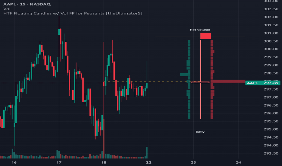
MFI Distribution [UAlgo]MFI Distribution is a statistics focused Money Flow Index indicator that combines a live MFI oscillator with a forward projected distribution histogram and normality diagnostics. Instead of only showing the current MFI line, the script collects a rolling history of MFI values, studies their distribution over a configurable lookback period, and visualizes the result as a histogram in the oscillator pane.
The indicator is designed for traders who want to understand how MFI behaves as a distribution , not only where it is on the current bar. It provides a compact statistical framework that helps answer questions such as:
Is MFI clustering around a narrow regime or spread across the full range
Is the recent MFI behavior skewed toward strong buying or selling pressure
Does the MFI sample look approximately normal, or is it fat tailed / asymmetric
How extreme is the current reading relative to the recent distribution
To support this, the script includes:
A live MFI line with dynamic gradient coloring
Overbought and oversold visual zones with gradient fills
A histogram of MFI frequency distribution over the selected lookback
An optional Gaussian curve overlay for visual comparison
A statistical dashboard with mean, standard deviation, skewness, kurtosis, and Jarque Bera normality test results
The histogram is drawn into the future area of the pane, so it does not interfere with the live MFI trace while still remaining visually aligned to the 0 to 100 oscillator scale.
Educational tool only. Not financial advice.
🔹 Features
🔸 1) Live MFI Oscillator with Regime Aware Coloring
The script plots a standard MFI line and colors it dynamically based on level behavior:
High MFI values transition toward red tones
Low MFI values transition toward green tones
Mid range values remain purple
This makes the oscillator easier to read at a glance, especially during sustained overbought or oversold conditions.
🔸 2) Overbought and Oversold Zone Visualization
The indicator includes standard MFI reference levels at 80 and 20, then adds gradient fills that become visible when the MFI pushes into extreme zones. This provides better visual emphasis for momentum extremes without cluttering the chart.
🔸 3) Rolling MFI History Collection for Statistical Analysis
The script maintains an internal array of the latest MFI values up to the user defined lookback length. This rolling sample is used to compute all distribution statistics and histogram frequencies on the last bar.
This design keeps the indicator responsive while ensuring the displayed distribution reflects the most recent market behavior.
🔸 4) Forward Projected MFI Distribution Histogram
A histogram is drawn in the oscillator pane using bins over the fixed MFI range from 0 to 100. Each bin counts how many MFI observations fall inside that interval during the lookback window.
The histogram is projected to the right of current price action in the pane, giving users a clean distribution panel without covering the live MFI line.
🔸 5) Configurable Histogram Resolution and Width
Users can control:
Lookback period used for distribution analysis
Number of histogram bins
Visual width of the histogram in future bars
This makes the tool flexible for both high level regime reading and finer distribution inspection.
🔸 6) Optional Gaussian Curve Overlay
When enabled, the script overlays a theoretical normal distribution curve using the sample mean and sample standard deviation. The curve is normalized to the histogram height so users can visually compare the empirical MFI distribution against a bell curve shape.
This is useful for quickly spotting asymmetry, multimodal clustering, or fat tail behavior.
🔸 7) Full Statistical Summary Dashboard
A built in dashboard table displays:
Mean
Standard Deviation
Skewness
Kurtosis (excess kurtosis)
Jarque Bera statistic
Pass / Fail normality status (95% threshold logic)
This turns the indicator into a compact quantitative diagnostic panel, not only a visual oscillator.
🔸 8) Jarque Bera Normality Test Classification
The script evaluates whether the MFI sample is approximately normal using a Jarque Bera style test and a fixed chi square threshold (95% confidence, 2 degrees of freedom). It then marks the result as PASS (Normal) or FAIL (Non Normal).
This helps traders distinguish between more stable oscillator regimes and structurally distorted ones.
🔸 9) Histogram Color Theme Based on Normality Result
The histogram automatically changes style depending on the test result:
Teal themed histogram when normality test passes
Red themed histogram when normality test fails
This creates an immediate visual signal of distribution quality without needing to read the dashboard first.
🔸 10) Last Bar Only Heavy Processing for Efficiency
Statistical calculations, histogram drawing, and dashboard refresh are performed only on the last bar. This reduces object churn and improves performance while preserving real time utility.
🔸 11) Object Based Drawing Management
The script uses custom types to organize logic:
DistributionStats for statistical values and normality output
HistoDrawer for histogram bars, curve lines, and labels
This makes the code structured and easier to extend with future features such as percentiles, z scores, or alternate tests.
🔹 Calculations
1) MFI Calculation
The script computes Money Flow Index from a user selected source and length:
mfi_val = ta.mfi(mfi_src, mfi_len)
This value is plotted in the oscillator pane and colored dynamically according to level.
2) Rolling History Buffer for Distribution Sampling
Each valid MFI value is pushed into a rolling array used for statistical analysis:
if not na(mfi_val)
mfi_history.push(mfi_val)
if mfi_history.size() > lookback
mfi_history.shift()
This ensures the sample size is capped at the selected lookback and continuously refreshed with recent values.
3) Sample Variance and Standard Deviation
The script computes sample variance using the classic n minus 1 denominator:
sum_sq_diff / (n - 1)
Standard deviation is then calculated as:
stats.stdev := math.sqrt(variance_val)
Using sample variance is appropriate here because the lookback window is treated as a sample of recent market behavior.
4) Sample Skewness Calculation
Skewness is computed from standardized deviations and corrected for sample size:
(n * sum_cube_diff) / ((n - 1) * (n - 2))
Interpretation:
Positive skew suggests more mass on lower values with a right tail toward high MFI prints
Negative skew suggests more mass on higher values with a left tail toward low MFI prints
5) Excess Kurtosis Calculation
The script calculates excess kurtosis , where a normal distribution is centered around 0:
float term1 = (n * (n + 1) * sum_quad_diff) / ((n - 1) * (n - 2) * (n - 3))
float term2 = (3 * math.pow(n - 1, 2)) / ((n - 2) * (n - 3))
term1 - term2
Interpretation:
Positive excess kurtosis suggests heavier tails or more peaked behavior
Negative excess kurtosis suggests flatter distribution behavior
6) Jarque Bera Normality Test
The script uses skewness and excess kurtosis to compute the Jarque Bera statistic:
stats.jb_stat := (n / 6.0) * (math.pow(stats.skew, 2) + 0.25 * math.pow(stats.kurt, 2))
Then it compares the result against a 95 percent chi square critical value (2 degrees of freedom):
stats.is_normal := stats.jb_stat < 5.991
Important note:
The code defines a jb_p_value field in the stats type, but this version does not explicitly calculate or display a p value. The pass / fail logic is threshold based.
7) Fixed MFI Range Histogram Binning (0 to 100)
The histogram always bins data over the full MFI range:
float min_val = 0.0
float max_val = 100.0
float bin_size = (max_val - min_val) / bins
Each MFI value is mapped to a bin index:
int bin_idx = math.floor(val / bin_size)
The index is clamped so values at boundaries stay valid:
if bin_idx >= bins
bin_idx := bins - 1
if bin_idx < 0
bin_idx := 0
This makes the histogram consistent across symbols and timeframes.
8) Frequency Counting and Peak Detection
For each binned MFI observation, the script increments a frequency counter and tracks the highest bin count:
int new_count = frequencies.get(bin_idx) + 1
frequencies.set(bin_idx, new_count)
if new_count > max_freq
max_freq := new_count
The maximum frequency is later used to normalize histogram bar heights.
9) Histogram Rendering Geometry
The histogram is drawn as boxes in the oscillator pane, projected to the right of the last bar:
int start_bar = bar_index + 5
float base_y = 10.0
float available_height = 80.0
This effectively uses the MFI pane vertical range from about 10 to 90 for histogram height visualization, keeping it aligned with the oscillator scale.
Each bin is mapped to x coordinates using its MFI interval and the user selected histogram width:
int x_left = start_bar + math.round((bin_val_start / 100.0) * chart_width_bars)
int x_right = start_bar + math.round((bin_val_end / 100.0) * chart_width_bars)
Each frequency is mapped to a vertical height using:
float bar_height_val = (freq / max_freq) * available_height
10) Histogram Color Logic from Normality Result
The histogram color theme is selected from the Jarque Bera pass / fail result:
Teal palette when stats.is_normal is true
Red palette when stats.is_normal is false
This creates a direct link between statistical classification and visual presentation.
11) Gaussian Curve Overlay Calculation
The script defines a normal probability density function:
(1.0 / (sigma * math.sqrt(2.0 * math.pi))) * math.exp(-0.5 * math.pow((x - mu) / sigma, 2))
For curve plotting:
It samples points across the histogram width
Maps each x position back to an MFI value from 0 to 100
Computes the PDF at that MFI value using the sample mean and standard deviation
Scales the PDF by the theoretical peak so the curve fits the histogram height
Key normalization idea:
float pdf_peak = normal_pdf(stats.mean, stats.mean, stats.stdev)
float current_y = base_y + (pdf_val / pdf_peak) * available_height
This makes the Gaussian curve visually comparable to the empirical histogram, even though one is a density and the other is raw frequency.
12) Dashboard Table Metrics
On the last bar, the script updates a table with the computed statistics:
Mean
StdDev
Skewness
Kurtosis
Jarque Bera statistic and normality classification
The result cell color changes based on normality:
Green for PASS (Normal)
Red for FAIL (Non Normal)
This gives traders a compact quantitative summary next to the visual distribution.
13) Overbought and Oversold Gradient Fills
The script adds gradient fills that appear when MFI moves beyond standard thresholds:
fill(plot_mfi, p_ob, 100, 80, ...)
fill(plot_mfi, p_os, 20, 0, ...)
This helps contextualize whether the current MFI reading is extreme while the histogram and dashboard describe the broader behavior of the recent MFI sample. Wskaźnik

Wskaźnik

Volume Flow Analysis [UAlgo]Volume Flow Analysis is a market profile style volume study that builds a session anchored volume distribution, extracts key reference levels from the previous profile, and generates institutional style context signals based on Auction Market Theory concepts. The script combines several workflows in one tool: previous session volume profile levels (POC, VAH, VAL), liquidity void detection through LVN valleys, acceptance versus rejection logic around value, and Initial Balance with open type classification.
The indicator runs on price ( overlay=true ) and is designed for intraday or swing traders who want a structured read of where value formed in the prior profile and how the current session is interacting with it. Instead of only plotting static lines, the script actively interprets behavior when price moves outside the previous value area. It checks whether the move is rejected quickly (failed auction) or sustained with time and volume (acceptance), which helps distinguish responsive activity from initiative activity.
Another major component is the profile shape and liquidity void framework. The script identifies previous profile shape as P, b, or D based on POC location within the profile range, and it scans for LVN valleys that can act as low participation zones where price may travel quickly. This gives the user both structural context and event based signals from the same indicator.
The result is a comprehensive volume flow dashboard that merges profile levels, session behavior, and AMT inspired signal logic into a single chart layer.
🔹 Features
🔸 1) Anchored Session Volume Profile (Daily, Weekly, Monthly or Custom Anchor)
The script builds a volume profile for each anchor period selected by the user through the Profile Period (Anchor) input. Common choices include Daily, Weekly, and Monthly anchors. When a new anchor session begins, the current session profile is finalized and promoted to the previous profile, then a new profile begins.
This allows the indicator to continuously reference the fully calculated previous profile while the current session is developing.
🔸 2) Price Range Binning with User Defined Resolution
Each session profile is divided into a configurable number of rows (bins). The script maps price activity into these bins and distributes volume proportionally based on the overlap between each candle range and each volume bin.
This creates a more realistic histogram than assigning all candle volume to a single price level, especially for wide range candles.
🔸 3) Previous Profile Core Levels (POC, VAH, VAL)
Once a session completes, the script calculates and stores the key profile levels:
POC (Point of Control), the price bin with the highest volume
VAH (Value Area High)
VAL (Value Area Low)
Value Area is computed by expanding outward from the POC until the chosen percentage of total profile volume is covered. These levels are then plotted on the chart as dynamic reference lines for the next session.
🔸 4) Acceptance vs Rejection Logic Around Previous Value Area
The indicator monitors current session behavior relative to the previous VAH and VAL and classifies behavior as either rejection (failed auction) or acceptance (initiative drive).
Failed Auction (Rejection):
Price trades outside the previous value area but returns back inside before meeting acceptance criteria. This is treated as a failed attempt to establish new value.
Acceptance (Initiative Drive):
Price stays outside the previous value area for a user defined number of bars and accumulates enough volume relative to average volume. This suggests successful acceptance of higher or lower value.
This framework is useful for separating temporary probes from meaningful value migration.
🔸 5) Institutional Style Signal Labels
The script can display signal labels for:
Failed Auction Bullish and Bearish
Acceptance Bullish and Bearish
LVN Traversal Bullish and Bearish
These labels appear directly on price and use user defined bullish and bearish colors for quick interpretation.
🔸 6) LVN Traversal (Liquidity Void / Vacuum) Detection
The script detects low volume nodes as true local valleys in the previous profile histogram. A bin qualifies as an LVN when surrounding bins on both sides have higher volume for a chosen valley depth.
If current price enters one of these prior LVN zones from above or below, the script marks a potential traversal event. This can help identify zones where price may move faster due to lower prior participation.
🔸 7) Previous Profile Shape Classification (P, b, D)
The script classifies the previous profile shape based on where the POC sits within the full profile range:
P shape if POC is near the upper portion of the profile
b shape if POC is near the lower portion
D shape if POC is near the middle
This gives quick context about the prior session structure, which can support directional bias interpretation and session planning.
🔸 8) Initial Balance (IB) Tracking
The indicator tracks the Initial Balance range using a user defined duration in minutes. During the IB window, it records session high and low. After the IB period ends, it can draw an IB box on the chart for visual reference.
This is useful for intraday frameworks where the IB range is used as a key reference for breakout, reversal, and auction development.
🔸 9) Open Type Classification and Daily Bias
At the start of each new anchor session, the script compares the new open to the previous value area and assigns a basic daily bias such as initiative bullish, initiative bearish, or responsive inside. After the IB period completes, it classifies the open type using rule based conditions, including:
Open Drive Bullish / Bearish
Open Rejection Reverse Bullish / Bearish
Open Test Drive Bullish / Bearish
This adds a session narrative layer on top of the profile levels.
🔸 10) Previous Profile Histogram Visualization on Last Bar
On the last bar, the script can render the previous profile histogram as a horizontal bar style distribution using boxes. Bins inside the previous value area can be colored differently from bins outside value.
This provides an at a glance visual summary of where prior volume concentrated, without needing a separate profile tool.
🔸 11) Extensive Visual Customization
Users can configure colors for:
Previous POC
Previous VA levels
Histogram bins
Value area histogram bins
Bullish signals
Bearish signals
This makes it easy to integrate the indicator into existing chart themes and workflows.
🔸 12) Structured Object Based Design
The script uses custom types ( VolumeBin and SessionProfile ) to store profile state, bins, levels, shape, and LVN zones. This object based approach keeps the logic modular and easier to maintain as features are added.
🔹 Calculations
1) Session Detection and Profile Lifecycle
A new profile session is detected with:
bool isNewSession = timeframe.change(i_anchor)
When a new session begins:
The current profile is finalized (end bar, profile calculations)
The current profile becomes the previous profile
A fresh session profile starts from the current bar
This design ensures that current session logic can reference a fully completed previous profile with stable POC, VAH, VAL, shape, and LVN data.
2) Volume Profile Bin Initialization
Each session profile is divided into i_rows equal price bins between session low and session high:
float step = (this.highestPrice - this.lowestPrice) / rows
for i = 0 to rows - 1
float bottom = this.lowestPrice + (i * step)
float top = bottom + step
this.bins.push(VolumeBin.new(top, bottom, 0.0))
As the current session high or low changes, the script rebuilds the current profile bins and repopulates volume from session start to the current bar. This keeps the current profile geometry aligned with the latest session range.
3) Proportional Volume Distribution Across Bins
For each candle, the script distributes volume across all bins according to candle range overlap:
float overlapTop = math.min(h, bin.priceTop)
float overlapBottom = math.max(l, bin.priceBottom)
if overlapTop > overlapBottom
float overlapRatio = (overlapTop - overlapBottom) / barRange
float volToAdd = v * overlapRatio
bin.volumeTotal += volToAdd
this.totalVolume += volToAdd
Interpretation:
Volume is allocated proportionally to the fraction of the candle range overlapping each price bin. This is a practical approximation of intrabar volume distribution across price.
Special handling exists for zero range candles, where volume is assigned to the bin containing the candle price.
4) POC Detection and Profile Max Volume
After session completion, the script scans all bins to find the highest volume bin:
for i = 0 to this.bins.size() - 1
VolumeBin bin = this.bins.get(i)
if bin.volumeTotal > maxVol
maxVol := bin.volumeTotal
pocIndex := i
The POC price is set to the midpoint of that bin:
this.pocPrice := (pocBin.priceTop + pocBin.priceBottom) / 2
The script also stores maxVolume , which is later used to scale histogram width display on the chart.
5) Value Area Calculation (VAH / VAL)
The Value Area is built by expanding outward from the POC until the target percentage of session volume is reached:
float targetVol = this.totalVolume * (vaPct / 100.0)
float currentVol = pocBin.volumeTotal
int upperIndex = pocIndex
int lowerIndex = pocIndex
At each step, the script compares the next upper and lower bin volumes and expands toward the larger volume side first. This continues until the cumulative value area volume reaches the target percentage.
Final levels:
this.vahPrice := this.bins.get(upperIndex).priceTop
this.valPrice := this.bins.get(lowerIndex).priceBottom
This is a standard volume profile style value area expansion method centered on POC.
6) Previous Profile Shape Classification (P, b, D)
The profile shape is inferred from the POC position inside the profile range:
float profileRange = this.highestPrice - this.lowestPrice
float pocPosPct = (this.pocPrice - this.lowestPrice) / profileRange
Classification logic:
P shape if POC is at or above 70 percent of the range
b shape if POC is at or below 30 percent
D shape otherwise
This is a simplified but practical shape proxy based on volume concentration location.
7) LVN (Liquidity Void) Valley Detection
The script identifies LVNs as local volume minima among profile bins, using a user defined valley depth i_lvnDepth . A bin is treated as an LVN if the bins on both sides for the specified depth all have greater volume:
for j = 1 to lvnDepth
if this.bins.get(i - j).volumeTotal <= currentBin.volumeTotal or this.bins.get(i + j).volumeTotal <= currentBin.volumeTotal
isValley := false
break
Only non zero volume bins are considered. Detected LVNs are stored in this.lvnZones for use in later traversal signals.
8) Initial Balance (IB) Calculation
At the start of a new session, the script resets IB state and starts tracking the session open, session start time, and current IB high and low. While the market is still inside the IB duration:
ibHigh := math.max(ibHigh, high)
ibLow := math.min(ibLow, low)
IB tracking ends once the elapsed time exceeds the configured duration in minutes:
if (time - sessionStartTime) >= i_ibMins * 60000
inIb := false
This produces the opening range used for later visualization and open type classification.
9) Daily Bias and Open Type Classification
At each new session open, the script sets a basic bias by comparing the session open to the previous value area:
Open above previous VAH suggests initiative bullish
Open below previous VAL suggests initiative bearish
Open inside previous value suggests responsive / inside
After the IB period ends, the script classifies the open type using rule based comparisons among:
Open location relative to previous VAH / VAL
Close relative to IB highs and lows
Intraday test and rejection behavior around prior value
Examples from the code include:
"Open-Drive Bullish"
"Open-Rejection-Reverse Bearish"
"Open-Test-Drive Bullish"
This gives a structured session narrative that aligns with many profile and AMT workflows.
10) Acceptance vs Failed Auction Logic (Above VAH)
The script tracks consecutive bars and cumulative volume when price closes above the previous VAH:
if close > prevVah
barsAboveVah += 1
volAboveVah += volume
If price returns inside value before acceptance is confirmed, it prints a failed auction bearish signal (fade breakout logic):
if barsAboveVah > 0 and not acceptedAbove and i_sigFailedAuc
isFailedAucBear := true
Acceptance bullish is confirmed only if both time and volume thresholds are satisfied:
if barsAboveVah >= i_accBars and volAboveVah >= (avgVol * i_accVolMult) and not acceptedAbove and i_sigAccept
acceptedAbove := true
isAcceptBull := true
This is a practical combination of time and participation filters, which reduces false acceptance signals from brief low volume excursions.
11) Acceptance vs Failed Auction Logic (Below VAL)
The same framework is applied below the previous VAL:
Tracking closes below VAL:
if close < prevVal
barsBelowVal += 1
volBelowVal += volume
Failed auction bullish if price returns inside before acceptance:
if barsBelowVal > 0 and not acceptedBelow and i_sigFailedAuc
isFailedAucBull := true
Acceptance bearish if time and volume thresholds are met:
if barsBelowVal >= i_accBars and volBelowVal >= (avgVol * i_accVolMult) and not acceptedBelow and i_sigAccept
acceptedBelow := true
isAcceptBear := true
This creates a symmetric AMT style signal model for both sides of value.
12) LVN Traversal Signal Logic
If LVN traversal signaling is enabled, the script checks whether price enters a previous LVN zone from outside:
Bullish traversal candidate when price enters the LVN from below
Bearish traversal candidate when price enters the LVN from above
Code logic example:
if close > lvn.priceBottom and close < lvn.priceTop and close < lvn.priceBottom
isLvnTravBull := true
This flags the moment price enters a potential liquidity void zone where faster movement may occur.
13) Previous Profile Histogram Rendering on Last Bar
On the last chart bar, the script draws the previous session histogram using boxes. Width is normalized by each bin volume relative to the profile max volume:
float widthRatio = bin.volumeTotal / previousProfile.maxVolume
int boxRight = bar_index + math.round((rightBar - bar_index) * widthRatio)
Bins inside VAH and VAL are colored using the value area histogram color, while other bins use the general histogram color. This gives a compact visual profile snapshot without external tools.
14) Dynamic Plots for Previous POC, VAH, and VAL
The previous profile reference levels are continuously plotted as line break style plots:
plot(plotPoc, "Prev POC", color=i_colPoc, linewidth=2, style=plot.style_linebr)
plot(plotVah, "Prev VAH", color=i_colVa, linewidth=1, style=plot.style_linebr)
plot(plotVal, "Prev VAL", color=i_colVa, linewidth=1, style=plot.style_linebr)
These lines provide stable reference levels throughout the current session and form the basis for the acceptance, rejection, and open type logic. Wskaźnik

Quantum Adaptive Session Profile v4Quantum Adaptive Session Profile (SVP) - The Dynamic Roadmap
Overview Traditional Volume Profiles and anchored VWAPs are incredibly useful, but they suffer from rigidity. When a market abruptly accelerates—like the New York session open on Gold or the Nasdaq—standard VWAP levels lag behind the true mean, leaving traders looking for pullbacks that never arrive. The Quantum Adaptive Session Profile (SVP) solves this by calculating a "Dynamic VWAP" using an Efficiency Ratio engine. The Point of Control (POC) and Value Areas automatically speed up to track explosive momentum, giving you real-time structural levels that actually respect the current market velocity.
Key Highlights
• The Adaptive Point of Control (POC): This acts as the session's dynamic fair value. During chop, it remains steady. When a breakout occurs, the alpha logic catches the volatility shift and aggressively pulls the POC to trail the new trend.
• Dynamic Value Areas (VAH / VAL): The Value Area High and Value Area Low expand and contract around the POC based on real-time standard deviations, mapping out the true "value" zone of the active session.
• Session Automation: Set your custom session hours in the inputs (e.g., London Open to NY Close). The indicator will automatically draw, track, and cleanly reset itself at the start of each new session to prevent historical data from polluting your current intraday levels.
• Fully Customizable Visuals: Take complete control over the colors and thickness of the POC, VAH, VAL, and background fill to match your personal chart aesthetic perfectly.
How to Trade It
1. The Range Market (Mean Reversion): When the Value Area bands are relatively flat, treat the VAH as resistance and the VAL as support. Fade the edges back toward the POC.
2. The Trend Market (Break & Retest): When price breaks strongly outside the VAH or VAL and the bands begin to aggressively angle upward/downward, the market is in price discovery mode. Do not fade this. Instead, wait for a pullback to the VAH (in an uptrend) or the VAL (in a downtrend) for continuation entries.
3. The Session Shift: Pay close attention to how price reacts to the POC during the first hour of your defined session. Staying above it implies buyer control for the day; staying below implies seller dominance.
The Quantum Ecosystem Integration
The Adaptive SVP is your structural roadmap on the main chart. It is designed to be paired with the Quantum sub-chart indicators for absolute precision:
1. Quantum Confluence : When price retraces to your Adaptive POC, look at Trendilo. If Trendilo flashes a Regular Divergence or glows Neon in the direction of the macro trend, you have a high-probability entry right off the structural level.
2. Quantum Z-Score : Combine VAH/VAL touches with extreme Z-Score readings (+2.0 / -2.0) to validate true exhaustion and snipe the reversal.
3. Quantum Main Chart Divergence: Use this to spot immediate structural momentum shifts exactly as price taps your SVP levels.
⚠️ DISCLAIMER: STRICTLY FOR EDUCATIONAL PURPOSES The information, scripts, and concepts provided in this publication are for educational and informational purposes only and do not constitute financial, investment, or trading advice. Trading in financial markets (including Forex, Crypto, Stocks, and Commodities) carries a high level of risk and may not be suitable for all investors. You could lose some or all of your initial investment. Past performance is not indicative of future results. Always conduct your own due diligence, backtest any strategy thoroughly, and consult with a certified financial advisor before making any trading decisions. By using this script, you acknowledge that you are solely responsible for your own trading actions and outcomes.
Wskaźnik

BK AK-Ghost Ladder👻 BK AK–Ghost Ladder — FVG Zones, Volume Profile, Confluence, Lifecycle 👻
🙏 All glory to G-d.
Built with standards and discipline passed down by my mentor — thank you for the relentless insistence on structure over noise, and for sharing real knowledge with generosity — no gatekeeping, no cheapness, no games.
Update / Record
A previous version of this publication was hidden due to insufficient description. This republish is a complete explanation of what the script does, how it works, how to use it, and what its limits are.
What this script does
Ghost Ladder is an overlay indicator that detects Fair Value Gaps (FVGs) and manages them as “living” support/resistance zones. It doesn’t just draw rectangles — it tracks each zone’s behavior (touches, breaks, role flips), grades strength (0–100), optionally builds an in-zone volume profile with POC, and adds confluence layers like pivots, MTF alignment, Fibonacci proximity, delta imbalance, sessions, and divergence warnings.
The goal is not prediction — it’s structured context: which zones matter, why they matter, and how price is interacting with them now.
Core features (what you’ll see on chart)
1) FVG detection (bull + bear)
Uses classic 3-bar gap logic:
Bullish FVG: low > high and gap size > ATR threshold
Bearish FVG: high < low and gap size > ATR threshold
Includes timeframe-adaptive distance filters (different settings under 1H vs ≥1H).
2) Zone lifecycle management
Each zone is stored and managed over time:
Expiration by max age (bars)
Optional “reset age on touch”
Optional overlap prevention / “keep strongest”
Optional proximity rules (minimum bars between zones)
“Clean mode” display (shifts/extends boxes for cleaner viewing)
3) Strength score (0–100) + ★ rating
Each zone gets a composite Strength Score that can include:
Volume vs average (optionally using lower timeframe volume aggregation)
Gap size vs ATR
Pivot confluence count
MTF confluence (additional timeframes)
Session weighting (Asia / London / NY / overlap)
Order block + imbalance checks
VWAP proximity/extreme bonus
Fib confluence
Delta divergence
Clustering / consolidation bonus
Role reversal bonus (support flips to resistance and confirms)
The star label displays score tiers (configurable thresholds):
★★, ★★★, ★★★★, ★★★★★
4) In-zone Volume Profile + POC (optional)
For each zone, Ghost Ladder can compute a lower-TF volume profile proxy inside the zone:
Configurable bins (resolution)
POC line (most volume concentration in-zone)
Optional total zone volume label
Optional delta coloring on POC (buy vs sell pressure)
Note: this is a practical proxy using lower-TF bar volumes/close locations — it is not exchange-level true volume-at-price.
5) Smart positioning / role logic (S/R behavior)
Optional “Smart Positioning” modes:
Show All
Hide Wrong Side
Auto Role Flip (support ↔ resistance based on price location + buffer)
Role reversal tracking:
Break detection (body break optional)
Break confirmation bars
Broken-zone persistence for N bars
Reactivation badge when zone becomes relevant again
6) Real-time divergence warnings (optional)
When price is interacting with a zone, it can flag divergence/weakness conditions using:
RSI divergence thresholding
OBV divergence (optional)
ADX weak-momentum check (optional)
You can choose how it displays:
Border only / icon only / both / color change
7) Fibonacci confluence (optional)
Computes fib levels from a lookback swing (highest/lowest over period), then counts if fib levels fall inside/near a zone (tolerance %). Optional fib lines + labels (with “only current fib” cleanup).
8) Adaptive learning + backtesting (optional)
Zones can be evaluated after touches:
“Success” if price moves away by a threshold
“Failure” if price violates beyond a threshold
Tracks wins/losses per zone
Updates an adaptive weight periodically
Optional ML-style confidence badge when sample size is meaningful
This is not a machine-learning model in the academic sense — it’s a performance-based weighting and confidence heuristic.
9) Info Table (optional)
A compact “war room” table on the last bar summarizing:
Active zone counts (bull vs bear)
Current market posture (near support/resistance, above/below, neutral)
Nearest S/R levels
Bias estimate
Active session
Risk assessment
10) Alerts
Built-in alert conditions include:
Magnetic pull active (price entering magnetic range of a strong zone)
Strong bullish FVG / strong bearish FVG (high strength score)
Divergence detected while price touches a zone
How to use (simple workflow)
Start with the stars: focus on ★★★★–★★★★★ zones first.
Trade the edges, not the middle: entries are usually better at zone boundaries with defined invalidation.
Respect role flips: a broken zone that flips and confirms can become a higher-quality level than a fresh gap.
Use divergence as a brake: divergence-at-zone = reduce size, wait for confirmation, or stand down.
Let filters remove excuses: tune distance filters, minimum stars, institutional-only mode, session weighting to match your market + timeframe.
Badge / icon legend (labels)
Depending on enabled features, labels may include:
🔥 = cluster / stacked zones
🎯 = pivot confluence
⚡ = MTF confluence
📐 = fib confluence
⚠ = delta divergence / warning
🔗 = merged / consolidated
📈 = upgraded to “institutional” classification
🤖 = confidence badge (sample-size based)
🔄 = reactivated zone
Repaint / reliability notes (important)
FVG zones: detected from past bars ( reference) → does not require future bars.
Pivot markers: use ta.pivothigh/ta.pivotlow → pivots confirm after pivotPeriod bars. That’s normal and means pivot signals are delayed/confirmed, not “future-looking.”
Lower-TF volume profile: depends on available lower timeframe data; can be heavier and may vary slightly by broker/feed.
Scores/labels: update as new touches, breaks, and confirmations occur (expected “living” behavior).
Performance / chart limits
This script uses many drawing objects (boxes/lines/labels) and can be resource-heavy:
Reduce profile bins, disable volume profile, or increase filters if you hit object limits or slowdowns.
“Clean Mode” can simplify the on-chart clutter.
Disclaimer
This indicator is for educational and analytical purposes only. It does not provide financial advice and does not guarantee outcomes. All “institutional / smart money / confidence” terminology is heuristic scoring, not a claim of certainty.
🙏 All glory to G-d — may He bless your vision, patience, and discipline at the boundary. Wskaźnik

HTF Candle Profile [UAlgo]HTF Candle Profile is a higher timeframe candle visualization tool that rebuilds each selected HTF candle from the lower timeframe bars that form it, then projects a horizontal volume profile inside that HTF candle range. The goal is to make intrabar participation visible directly on the price chart, so you can see where volume concentrated within the candle, where it was thin, and where the dominant traded price level emerged.
Instead of treating a daily or four hour candle as a single block, the script aggregates the lower timeframe bars as they arrive and distributes their volume across price bins covering the HTF candle’s high to low range. The result is a compact profile drawn from the start time of the HTF candle toward the right, with width proportional to relative volume per bin and color intensity driven by a gradient. This provides a fast read of internal structure: balanced candles, directional candles, rejection wicks, and consolidation pockets become easier to interpret because you can see the volume distribution inside the candle.
The indicator draws on the main chart and keeps a small rolling history of recent HTF candles to stay responsive and to respect object limits.
🔹 Features
1) Multi Timeframe HTF Candle Reconstruction
The script listens for a new HTF candle event using the selected timeframe input. When a new HTF candle begins, the previous one is finalized and drawn. During the active HTF candle, each incoming lower timeframe bar updates the running OHLC and stores its high, low, and volume for profiling.
This approach enables a live building profile for the current HTF candle while preserving completed profiles for recent candles.
2) Intrabar Volume Profile Built from LTF Data
For each HTF candle, the price range from low to high is divided into a user defined number of bins. Each lower timeframe bar contributes volume into all bins it spans. Volume is distributed evenly across the spanned bins to approximate participation within that bar’s range. This produces a per bin volume distribution that is stable and visually interpretable even when lower timeframe candles have large ranges.
3) Gradient Based Profile Intensity
Each bin is drawn as a horizontal box. Its color comes from a gradient that maps low volume to a softer profile color and high volume to a stronger profile color. This makes it easy to spot high participation nodes and low participation voids within the HTF candle.
Inputs allow independent control for bullish and bearish candle coloring and for the low volume and high volume profile colors.
4) POC Line Option
The script can optionally plot a POC line representing the price level of maximum volume within the HTF candle. This is drawn as a dashed horizontal line that spans the candle’s start time to end time. POC is often used as a reference for acceptance, fair value, or a magnet level during retracements.
5) Candle Body, Wick, and Time Boundaries
To keep the profile anchored and readable, the script also draws:
A translucent body box from HTF open to HTF close
A vertical wick line from HTF high to HTF low
A dotted start boundary and a dotted end boundary for the HTF candle window
These elements provide context so the profile is always interpreted within the candle structure that produced it.
6) Object Management and Rolling History
To keep charts clean and avoid exceeding platform limits, the script maintains a small history of HTF candles and deletes drawings for older ones. Each candle owns its objects and can fully clear them when removed from the rolling window.
🔹 Calculations
1) New HTF Candle Detection
A new candle event is detected using timeframe change on the selected timeframe:
isNew = timeframe.change(tf)
When isNew is true:
The previous HTF candle is finalized by setting its end time and drawing it
A new HTF candle object is created and added to the array
Old candles beyond the history limit are removed and their drawings deleted
2) HTF Candle Aggregation from LTF Bars
Each incoming lower timeframe bar updates the active HTF candle:
method addLtf(HtfCandle this, float h, float l, float c, float v) =>
this.ltfData.push(LtfBar.new(h, l, v))
this.h := math.max(this.h, h)
this.l := math.min(this.l, l)
this.c := c
Interpretation:
High is updated to the maximum seen so far within the HTF candle window
Low is updated to the minimum seen so far
Close is updated to the most recent close
Each LTF bar is stored with its high, low, and volume for later bin distribution
3) Bin Construction Across the HTF Candle Range
When drawing a candle, the script divides the HTF range into binCount segments:
float step = (this.h - this.l) / bCount
for i = 0 to bCount - 1
this.bins.push(ProfileData.new(this.l + i * step, this.l + (i + 1) * step, 0.0, na))
Each bin stores:
minP and maxP boundaries
accumulated volume for that price segment
a box handle for drawing
4) Volume Distribution from Each LTF Bar into Bins
For each stored LTF bar, the script determines which bins the bar spans and distributes volume evenly across them:
int startIdx = int((ltf.l - this.l) / step)
int endIdx = int((ltf.h - this.l) / step)
startIdx := math.max(0, math.min(startIdx, bCount - 1))
endIdx := math.max(0, math.min(endIdx, bCount - 1))
int spanned = endIdx - startIdx + 1
float vPerBin = ltf.v / spanned
for j = startIdx to endIdx
ProfileData b = this.bins.get(j)
b.vol += vPerBin
Interpretation:
The bar range is mapped to bin indexes
Indexes are clamped so they remain inside the array
Volume is divided by the number of spanned bins
Each spanned bin receives an equal share of that bar’s volume
This is a robust approach for intrabar profiling without tick data.
5) POC Computation
The script finds the bin with the maximum accumulated volume and sets the POC price at the midpoint of that bin:
float maxVol = 0.0
float pocP = na
for b in this.bins
if b.vol > maxVol
maxVol := b.vol
pocP := math.avg(b.minP, b.maxP)
If enabled, a dashed POC line is drawn across the HTF candle window:
if sPoc and not na(pocP)
this.lPoc := line.new(x1=this.st, y1=pocP, x2=this.et, y2=pocP, xloc=xloc.bar_time, color=cPoc, style=line.style_dashed, width=2)
6) Profile Box Width Scaling
Each bin’s box width scales by its volume relative to the maximum volume bin. Width is capped as a fraction of the candle’s time duration:
int duration = math.max(this.et - this.st, 1)
int volWidth = int((duration * 0.40) * (b.vol / maxVol))
int boxRight = this.st + volWidth
Interpretation:
duration represents the HTF candle time width
0.40 is the maximum profile width fraction of the candle duration
b.vol / maxVol converts volume to a normalized ratio
boxRight is calculated so all profile boxes start at the candle start time and extend rightward based on volume
7) Gradient Coloring of the Profile
Each bin color is mapped from low volume to high volume using a gradient:
color gradColor = color.from_gradient(b.vol, 0, maxVol, cLow, cHigh)
This keeps low participation zones visually lighter and high participation zones more prominent.
8) Candle Body and Wick Drawing
The script draws an HTF candle body box and a wick line for context:
float topP = math.max(this.o, this.c)
float botP = math.min(this.o, this.c)
this.bBody := box.new(left=this.st, top=topP, right=this.et, bottom=botP, xloc=xloc.bar_time, bgcolor=color.new(c, 85))
this.lWick := line.new(x1=midTime, y1=this.h, x2=midTime, y2=this.l, xloc=xloc.bar_time, color=color.new(c, 30), width=2)
It also draws start and end boundary lines so the candle window is clearly defined in time.
Wskaźnik

Delta Ladder Order Flow [UAlgo]Delta Ladder Order Flow is an overlay order flow visualizer that builds a per bar delta ladder using lower timeframe candles as an intrabar proxy. For each recent bar, the script pulls the underlying lower timeframe open, high, low, close, and volume arrays, then distributes volume into discrete price buckets. Each bucket accumulates estimated buy volume and sell volume, producing a ladder that resembles a footprint style view.
The display focuses on three core outputs:
A delta heatmap ladder where each price level is colored by net delta dominance
A Point of Control highlight that marks the highest total volume level inside the bar
A stacked imbalance detector that scans diagonally across levels to identify aggressive one sided participation and optionally projects that stack forward
The system is designed with stability controls for real world chart conditions. It includes dynamic scaling to prevent excessive level counts on high range bars, object budgeting through bars to draw limits, and text filtering to reduce clutter.
🔹 Features
1) Intrabar Resolution via Lower Timeframe Data
The ladder is constructed using request.security_lower_tf. You select an Intrabar Resolution timeframe that must be lower than the chart timeframe. The script then receives arrays of LTF candles for each chart bar and uses them as a proxy for footprint style aggregation.
This approach provides a practical order flow approximation on TradingView charts without requiring native tick level data.
2) Ladder Aggregation with Tick Size Multiplier
Price levels are aggregated using the symbol mintick multiplied by a user multiplier. Increasing the multiplier produces thicker ladder steps and fewer levels. Decreasing it produces finer granularity but increases the number of boxes drawn.
This control is critical for balancing detail versus performance across different symbols and volatility regimes.
3) Dynamic Scaling to Prevent High Range Bar Overload
A single volatile bar can contain too many price steps if the granularity is too fine. To prevent crashes, the script estimates how many steps would be required for the bar and increases the effective step size when the raw step count exceeds Max Levels per Bar.
This keeps rendering stable even during high volatility events while still maintaining a consistent ladder representation.
4) Buy, Sell, and Neutral Volume Attribution
Each LTF candle’s direction is inferred from its open and close:
Close above open is treated as buy side volume
Close below open is treated as sell side volume
Close equal open is treated as neutral and split evenly between buy and sell
Volume is then distributed across the price buckets covered by the LTF candle range so that wide candles spread their influence across multiple levels.
5) Delta Heatmap Ladder with Intensity Scaling
Each price bucket computes delta as buy volume minus sell volume and total volume as the sum of both. Ladder cells are colored positive or negative based on delta sign, and transparency is scaled by how dominant the delta is relative to the maximum total volume level inside that bar. This yields a compact heatmap where strong imbalances visually stand out.
A square root curve is applied to intensity to improve mid tone visibility without making everything fully opaque.
6) Point of Control Highlight
The ladder tracks the price level with the highest total volume and marks it as the Point of Control. When enabled, the POC row uses a dedicated border color and a stronger border width so the acceptance anchor is immediately visible.
7) Stacked Imbalance Detection and Projection
The script can detect stacked diagonal imbalances. It compares volume across adjacent price levels using a diagonal logic similar to footprint tools:
Bullish diagonal checks buy volume at a level versus sell volume at the level below
Bearish diagonal checks sell volume at a level versus buy volume at the level above
An imbalance requires the winning side to exceed the losing side by the configured Imbalance Ratio and also exceed a minimum volume threshold to filter low volume noise. When consecutive imbalanced levels reach the Stacked Levels count, the stack is marked and optionally extended forward as a zone.
Stack members also override normal heatmap coloring and are rendered more solid for emphasis.
8) Clean Visual Controls
Several options support readability:
Bars to Draw limits workload and object count
Show Delta Values can be toggled on or off
Min Delta to Show Text filters small prints
Ladder Width percent controls how wide the ladder is relative to the bar space
Text size can be adjusted for different chart zoom levels
Box outline can be hidden by default for a cleaner footprint aesthetic
🔹 Calculations
1) Intrabar data acquisition (lower timeframe arrays)
The script requests arrays of LTF OHLCV values for each chart bar using request.security_lower_tf.
ltf_open = request.security_lower_tf(syminfo.tickerid, tf_input, open)
ltf_close = request.security_lower_tf(syminfo.tickerid, tf_input, close)
ltf_high = request.security_lower_tf(syminfo.tickerid, tf_input, high)
ltf_low = request.security_lower_tf(syminfo.tickerid, tf_input, low)
ltf_vol = request.security_lower_tf(syminfo.tickerid, tf_input, volume)
These arrays contain the lower timeframe candles that make up each chart bar. Each chart bar index has its own embedded array.
2) Base tick step (bucket size control)
Bucket size starts from mintick multiplied by Tick Size Multiplier.
var float base_tick_step = syminfo.mintick * tick_size_mult
This is the baseline price increment used to build the ladder levels.
3) Last bar execution model (performance design)
The script only builds and draws ladders when barstate.islast is true. It then reconstructs the last N bars using an index offset.
if barstate.islast
int start_idx = math.max(0, bar_index - bars_to_draw + 1)
for i = start_idx to bar_index
int offset = bar_index - i
float arr_o = ltf_open
float arr_c = ltf_close
float arr_h = ltf_high
float arr_l = ltf_low
float arr_v = ltf_vol
This design dramatically reduces CPU and memory load compared to updating every bar.
4) Dynamic scaling per bar (anti crash protection)
For each bar, the script estimates how many price steps would be needed using the current bucket size. If that count exceeds Max Levels per Bar, it increases the step size only for that bar.
float bar_h = high
float bar_l = low
float bar_range = bar_h - bar_l
float raw_steps = bar_range / base_tick_step
int scaler = 1
if raw_steps > max_levels_per_bar
scaler := int(math.ceil(raw_steps / max_levels_per_bar))
float current_tick_step = base_tick_step * scaler
Result:
Calm bars use fine granularity
High range bars are automatically compressed into fewer buckets
5) LTF candle direction classification (buy, sell, neutral)
Each LTF candle is classified using its open and close. Neutral candles split volume evenly.
bool is_buy = c > o
bool is_sell = c < o
bool is_neutral = c == o
This is a heuristic proxy for aggressor side. It is not true bid ask data.
6) Align LTF candle range to bucket grid
The candle low and high are rounded to the current tick step so bucket prices align cleanly.
float low_aligned = math.round(l / current_tick_step) * current_tick_step
float high_aligned = math.round(h / current_tick_step) * current_tick_step
7) Step counting and volume per step
The script computes how many bucket levels the candle touches and divides volume equally across them.
int steps = int(math.round((high_aligned - low_aligned) / current_tick_step)) + 1
if steps > 500
steps := 500
float vol_per_step = v / steps
This means wide candles distribute volume across more ladder cells, while tight candles concentrate volume into fewer cells.
8) Writing volume into the ladder map (PriceLevel storage)
Each chart bar owns a DeltaLadder with a map of price to PriceLevel. Each PriceLevel stores buy and sell volume. Volume is added step by step.
type PriceLevel
float price
float buy_vol = 0.0
float sell_vol = 0.0
type DeltaLadder
int bar_idx
map levels
float min_price = 10000000.0
float max_price = 0.0
float max_vol_level = 0.0
float poc_price = na
float poc_vol = 0.0
The add method updates volumes and also tracks max volume and POC:
method add_volume(DeltaLadder this, float price, float vol, bool is_buy, bool is_neutral) =>
if not this.levels.contains(price)
this.levels.put(price, PriceLevel.new(price))
PriceLevel lvl = this.levels.get(price)
if is_neutral
lvl.buy_vol += vol * 0.5
lvl.sell_vol += vol * 0.5
else if is_buy
lvl.buy_vol += vol
else
lvl.sell_vol += vol
float t = lvl.total()
if t > this.max_vol_level
this.max_vol_level := t
if t > this.poc_vol
this.poc_vol := t
this.poc_price := price
The main loop calls this method for each bucket level touched by each LTF candle:
for p = 0 to steps - 1
float level_price = low_aligned + (p * current_tick_step)
ladder.add_volume(level_price, vol_per_step, is_buy, is_neutral)
9) Delta and total volume formulas
Delta and total are defined as methods on PriceLevel.
method delta(PriceLevel this) =>
this.buy_vol - this.sell_vol
method total(PriceLevel this) =>
this.buy_vol + this.sell_vol
These values drive both coloring and POC selection.
10) Stacked imbalance detection (diagonal footprint logic)
Prices are sorted so neighbor comparisons are correct. A stack_map stores whether each price belongs to a bullish or bearish stacked run.
float prices = ladder.levels.keys()
array.sort(prices)
map stack_map = map.new()
Diagonal comparisons:
Bullish diagonal compares BuyVol at level i with SellVol at level below i minus 1
Bearish diagonal compares SellVol at level i with BuyVol at level above i plus 1
Bullish check includes a zero handling rule:
if i > 0
float p_below = array.get(prices, i-1)
PriceLevel lvl_below = ladder.levels.get(p_below)
if lvl_below.sell_vol == 0
if lvl.buy_vol > imb_min_vol
direction := 1
else
if lvl.buy_vol > lvl_below.sell_vol * imb_ratio and lvl.buy_vol > imb_min_vol
direction := 1
Bearish check includes symmetric logic:
if i < array.size(prices) - 1
float p_above = array.get(prices, i+1)
PriceLevel lvl_above = ladder.levels.get(p_above)
if lvl_above.buy_vol == 0
if lvl.sell_vol > imb_min_vol
direction := -1
else
if lvl.sell_vol > lvl_above.buy_vol * imb_ratio and lvl.sell_vol > imb_min_vol
direction := -1
Runs are tracked and only accepted if the number of consecutive levels meets the stacked requirement:
if math.abs(i - run_start_idx) >= stack_count
for k = run_start_idx to i - 1
stack_map.put(array.get(prices, k), run_dir)
The script also draws a projected zone for the detected stack band:
box.new(right_time, p_top + current_tick_step/2, right_time + 1000 * 60 * 60 * 24, p_bot - current_tick_step/2,
xloc=xloc.bar_time, border_width=0, bgcolor=color.new(c_stack, 85), extend=extend.right)
11) Heatmap intensity and transparency mapping
For each price level, intensity is computed as abs(delta) relative to the maximum total volume level in the bar, then curved and mapped into transparency.
float intensity = ladder.max_vol_level > 0 ? math.abs(delta) / ladder.max_vol_level : 0
intensity := math.min(intensity, 1.0)
float curved_intensity = math.sqrt(intensity)
float transp = 97 - (curved_intensity * 57)
Stacked members force stronger visibility:
if stack_map.contains(p)
intensity := 1.0
transp := 30
12) POC marking in the drawing pass
POC is detected during volume accumulation, then used in rendering to upgrade the border style for that cell.
bool is_poc = show_poc and (p == ladder.poc_price)
color border_c = is_poc ? col_poc : col_outline
int border_w = is_poc ? 2 : 1
13) Delta text rendering filter
Text labels are optional and can be filtered by a minimum absolute delta threshold.
if show_text and math.abs(delta) >= text_threshold
string txt = str.tostring(delta, format.volume)
label.new(int((left_time + right_time)/2), p, txt,
xloc=xloc.bar_time, style=label.style_none,
textcolor=txt_col, size=text_size)
Wskaźnik
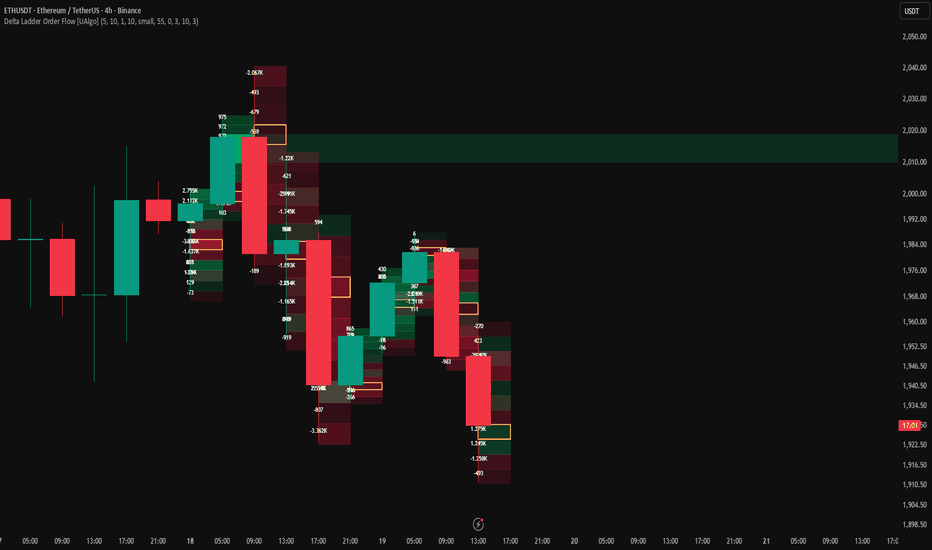
Accumulation Zone Profiles [UAlgo]Accumulation Zone Profiles is an overlay indicator that detects low volatility accumulation phases and automatically builds a fixed range volume profile for each confirmed zone. The script uses a statistical volatility model based on log returns, identifies periods where volatility compresses into an unusually quiet regime, then verifies that price action remains sufficiently sideways before confirming the zone.
When a zone is confirmed, the indicator draws two complementary views:
A highlighted accumulation range on the chart
A fixed range volume profile drawn to the right of the zone, including Point of Control and Value Area levels
The intent is to turn consolidation into a structured map. Instead of treating ranges as vague rectangles, the script assigns a volume distribution to the range so you can see where the market accepted price, where it rejected price, and which levels are most likely to matter during expansion.
🔹 Features
1) Statistical Accumulation Detection Using Log Volatility
The detection engine starts from log returns r = ln(C / C ) and builds an EWMA based volatility estimate. Volatility is converted into log space and evaluated with a rolling distribution model. A z score determines whether the current volatility is unusually low relative to its own history.
Zones begin when the z score falls below a configurable entry threshold and they end after volatility recovers above an exit threshold for a configurable number of confirmation bars.
2) Sideways Quality Filter With Trend Score
Not every low volatility period is true accumulation. The script measures drift using a trend score defined as:
absolute sum of returns divided by sum of absolute returns
Lower values indicate more rotation and less directional drift. A maximum trend score filter ensures zones remain meaningfully sideways before a profile is created.
3) Non Repainting Option Using Confirmed Bars
When enabled, the system only updates on confirmed bars. This reduces repainting behavior and makes zone start and zone end decisions more stable for live trading workflows.
4) Fixed Range Volume Profile Per Zone
For each confirmed accumulation zone, the script builds a histogram of volume across a user selected number of price rows. Each bar’s volume is distributed into bins according to how much of that candle range overlaps each bin. This produces a true fixed range profile for the zone.
The profile is drawn to the right of the zone so it does not cover price action.
5) Point of Control and Value Area Levels
The highest volume row is treated as the Point of Control. Value Area High and Value Area Low are computed by expanding outward from POC until a target percent of total volume is captured. This creates a practical acceptance framework inside the zone.
Optional plotting allows:
Highlighting the POC row
Drawing VAH and VAL lines
Drawing zone boundary guides
Showing an information label that summarizes zone statistics
6) Tick Alignment For Clean Levels
If enabled, the zone range, bin step size, and derived levels are aligned to the instrument tick size. This produces cleaner price levels and reduces floating point noise in labels and lines.
7) Object Budget Management
Volume profiles use many boxes. The script computes an effective rows value based on the number of profiles you choose to keep, then limits total box usage so you are less likely to hit platform object limits. Older profiles are deleted automatically when new ones are created.
8) Alerts
Two alerts are available:
Accumulation Zone Started
Accumulation Zone Confirmed and Profile Created
This supports automation such as watchlist monitoring and breakout preparation.
🔹 Calculations
1) Log Return and EWMA Variance
The script defines log return as ln(C / C ) and uses an EWMA of squared returns as a variance proxy.
Alpha for EWMA:
f_alpha(int len) =>
2.0 / (len + 1.0)
Log return:
lr = math.log(close / close )
lr := na(close ) or close == 0.0 ? 0.0 : lr
EWMA variance and volatility:
alphaFast = f_alpha(fastLen)
var float ewmaVarR = na
ewmaVarR := na(ewmaVarR ) ? lr * lr : alphaFast * (lr * lr) + (1.0 - alphaFast) * ewmaVarR
vol = math.sqrt(math.max(ewmaVarR, 0.0))
2) Log Volatility Distribution and z Score
Volatility is transformed into log space to stabilize distribution behavior. The script maintains EWMA estimates of mean and second moment, then computes standard deviation and z score.
eps = 1e-10
logVol = math.log(vol + eps)
alphaDist = f_alpha(distLen)
var float m1 = na
var float m2 = na
m1 := na(m1 ) ? logVol : alphaDist * logVol + (1.0 - alphaDist) * m1
m2 := na(m2 ) ? logVol * logVol : alphaDist * (logVol * logVol) + (1.0 - alphaDist) * m2
sigma = math.sqrt(math.max(m2 - m1 * m1, eps))
z = (logVol - m1) / sigma
Interpretation:
Negative z means volatility is below its typical level
More negative z means stronger compression
3) Zone Start and Zone End Conditions
Entry and exit logic uses the z score relative to thresholds:
Start when z is less than or equal to minus Enter Threshold
End when z is greater than or equal to minus Exit Threshold for Exit Confirm Bars
lowNow = not na(z) and z <= -enterZ
highNow = not na(z) and z >= -exitZ
Exit confirmation counter:
zb.exitCount := highNow ? zb.exitCount + 1 : 0
bool exitByConfirm = zb.exitCount >= exitBars
A maximum zone duration also forces closure:
bool exitByMax = zb.barCount() >= maxZoneBars
If exit is triggered via confirmation bars, the script removes those last bars from the zone before profiling to avoid contaminating the accumulation range with the volatility recovery phase.
4) Sideways Drift Score Filter
During zone building, returns are accumulated:
sumR is the signed drift
sumAbsR is total movement magnitude
Trend score:
method driftScore(ZoneBuilder this) =>
math.abs(this.sumR) / math.max(this.sumAbsR, 1e-10)
A zone is accepted only if:
Bar count is at least Min Zone Bars
Drift score is less than or equal to Max Trend Score
5) Profile Range and Row Step
Once accepted, the profile range is built from the min low and max high of the zone. The range is optionally aligned to tick.
Step size equals range divided by rows, with optional tick alignment:
float stepRaw = (hi - lo) / rows
float step = stepRaw
if alignTick
step := math.max(syminfo.mintick, f_roundToTick(stepRaw))
6) Volume Histogram Construction
For each bar in the zone, volume is assigned into bins.
If the candle range is very small, volume goes to a single nearest bin.
Otherwise, volume is distributed proportionally by overlap between candle range and each bin range.
Core proportional distribution logic:
float overlap = math.max(0.0, math.min(bh, binHi) - math.max(bl, binLo))
if overlap > 0
float frac = overlap / br
array.set(binVol, b, array.get(binVol, b) + bv * frac)
This produces binVol, a per row volume distribution.
7) POC Calculation
POC is the index of the maximum bin volume. POC price is the center of that row.
if v > maxV
maxV := v
pocIdx := b
float poc = lo + (pocIdx + 0.5) * step
8) Value Area Computation
Value Area is derived by expanding outward from POC until the cumulative volume reaches Value Area percent of total volume.
Target volume:
float target = totV * (valueAreaPct / 100.0)
Expand left and right by choosing the side with higher next volume until the target is met. This creates a contiguous value area band.
VAL and VAH mapping to prices:
float valP = lo + left * step
float vahP = lo + (right + 1) * step
9) Rendering Logic
Zone highlight is drawn directly over the accumulation period using a box with configurable fill and border transparency.
The volume profile is drawn as a stack of boxes to the right of the zone. Each row width is proportional to row volume relative to max row volume. Transparency is mapped so high volume rows appear more prominent.
POC row can be highlighted using a dedicated color and transparency configuration.
VAH and VAL can be drawn as horizontal lines across the profile region, and optional boundary lines can mark the start and end of the detected zone.
10) Profile Retention and Cleanup
Profiles are stored in an array. When the number of stored profiles exceeds Keep Last Profiles, the oldest profile is deleted and all of its objects are removed. This keeps the chart responsive and prevents reaching the platform maximum object counts. Wskaźnik