
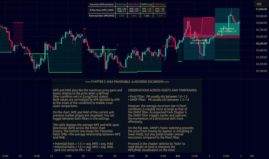
Hello everyone. I compared Pivot States vs. OMSF-Engulfing using MFE (Maximum Favorable Excursion), MAE (Maximum Adverse Excursion), and the resulting Potential Ratio (PR) (Learning Space, Chapter 5).
TL;DR:
MFE and MAE measure the maximum price movements during a defined market state in the expected and adverse directions, respectively. The MFE/MAE ratio (Potential Ratio) describes profit potential relative to drawdown potential. The results:
The results reflect the findings from the KER section and highlight the descriptive, stable
character of Pivot High/Low signals, whereas OMSF-Engulfing shows potential as a viable entry signal.
First, a fundamental note: I am not sure if this has been entirely clear up to this point—strictly speaking, neither Pivot States nor OMSF-Engulfing can yet be considered true "trend filters" (see figures below). Both approaches have primarily served to illustrate and compare the basic concepts of "Pivot Points" vs. "OMSF Structure" in a measurable way.
1. Methodology
State Logic
As a reminder: Both indicators (Pivots and OMSF) have two states. When a Pivot or OMSF Low is confirmed, the "Long" state begins. When a High is confirmed, the indicator switches to "Short", simultaneously ending the Long state (and vice versa).
Calculation of Table Values
When a state ends (e.g., Long), the counter for Long states increases by 1. The MFE and MAE values achieved during this phase are added to the respective totals. From this, the average table values are calculated:
ATR Normalization
On the first bar of a new state, the current ATR(14) is saved as a fixed "Start ATR". As long as this state remains active, the continuously measured MFE and MAE values are divided by this exact Start ATR. This offers two key advantages:
2. Results and Interpretation
Let's look at the concrete observations across various assets and timeframes:
⚠️ Note: I manually clicked through various assets and timeframes on the chart and observed the values in the tables. The underlying pattern remains remarkably consistent across different markets. Therefore, the numbers listed here are rough, "eyeballed" estimates from these samples rather than scientifically calculated global averages across a massive database 😉.
Price Movement Excursion: The average MFE for Pivot conditions is roughly twice as large as that of OMSF. Pivot structures remain active longer and capture larger, higher-timeframe swings.
Adverse Excursion (MAE): The faster switching of OMSF-Engulfing effectively prevents price from moving far against the initial direction after a signal. MAE is substantially lower at 1.1–1.2 compared to the slower Pivots (2.0–2.3).
Momentum and Potential Ratio: As expected from the Kaufman Efficiency Ratio (KER) chapter, OMSF triggers earlier, capturing directional momentum more quickly. Overall, this results in smaller price excursions (MFE) but also lower drawdowns (MAE), leading to a more favorable average Potential Ratio (1.3 to 1.6). For Pivot States, deeper drawdowns pull this ratio toward a neutral 1:1 value.
Advantage OMSF Engulfing:
Advantage Pivot States:
3. A Reality Check on MFE & MAE
A complete trading setup cannot be derived directly from these values. There are two main reasons for this:
1. The Reality of Exits
MFE measures the theoretical maximum price movement during a state. In practice, no one consistently hits the absolute top or bottom of a move. Exits are always a compromise: you either take profits too early or give back gains after the peak. The theoretical potential of MFE can never be fully captured in real markets.
[b]2. Statistical Distribution (Average vs. Reality)
A simple mean can draw a heavily skewed picture. Analyzing the actual distribution of MFE and MAE reveals significant asymmetry: a few extreme outliers pull the calculated average upward.
In practice, the calculated average value corresponds roughly to the 66th percentile. Specifically, this means that only in about one-third of all cases (approx. 33%) is this mathematical average value reached or exceeded.
Thus, the average values primarily serve as a relative point of comparison between concepts. However, I wondered whether the specific excursion distribution could be used—for instance, to systematically set stop-loss levels (via MAE percentiles) or take-profits (below MFE percentiles). I built a small research tool for this purpose. Once the tool is presentable and properly documented, I will share it here.
Best regards,
arni
TL;DR:
MFE and MAE measure the maximum price movements during a defined market state in the expected and adverse directions, respectively. The MFE/MAE ratio (Potential Ratio) describes profit potential relative to drawdown potential. The results:
- OMSF-Engulfing shows significantly smaller excursions than Pivot States.
- OMSF-Engulfing yields an average positive Potential Ratio.
- The Potential Ratio of Pivot States is lower and tends toward 1:1.
The results reflect the findings from the KER section and highlight the descriptive, stable
character of Pivot High/Low signals, whereas OMSF-Engulfing shows potential as a viable entry signal.
First, a fundamental note: I am not sure if this has been entirely clear up to this point—strictly speaking, neither Pivot States nor OMSF-Engulfing can yet be considered true "trend filters" (see figures below). Both approaches have primarily served to illustrate and compare the basic concepts of "Pivot Points" vs. "OMSF Structure" in a measurable way.
1. Methodology
State Logic
As a reminder: Both indicators (Pivots and OMSF) have two states. When a Pivot or OMSF Low is confirmed, the "Long" state begins. When a High is confirmed, the indicator switches to "Short", simultaneously ending the Long state (and vice versa).
Calculation of Table Values
When a state ends (e.g., Long), the counter for Long states increases by 1. The MFE and MAE values achieved during this phase are added to the respective totals. From this, the average table values are calculated:
- avg. MFE = Total MFE / Number of States
- avg. PR (Potential Ratio) = avg. MFE / avg. MAE
ATR Normalization
On the first bar of a new state, the current ATR(14) is saved as a fixed "Start ATR". As long as this state remains active, the continuously measured MFE and MAE values are divided by this exact Start ATR. This offers two key advantages:
- It makes values comparable across different assets and timeframes.
- In practice, traders usually set their stop losses relative to current volatility. Through normalization, the Potential Ratio (PR) provides a metric strongly reminiscent of the classic Risk-Reward Ratio (RRR) and is intuitively understandable.
2. Results and Interpretation
Let's look at the concrete observations across various assets and timeframes:
- Pivot-Condition: avg. MFE 2.5–3.0 | avg. MAE 2.0–2.3 | avg. PR 1.0–1.3
- OMSF-Engulfing: avg. MFE 1.3–1.8 | avg. MAE 1.1–1.2 | avg. PR 1.3–1.6
⚠️ Note: I manually clicked through various assets and timeframes on the chart and observed the values in the tables. The underlying pattern remains remarkably consistent across different markets. Therefore, the numbers listed here are rough, "eyeballed" estimates from these samples rather than scientifically calculated global averages across a massive database 😉.
Price Movement Excursion: The average MFE for Pivot conditions is roughly twice as large as that of OMSF. Pivot structures remain active longer and capture larger, higher-timeframe swings.
Adverse Excursion (MAE): The faster switching of OMSF-Engulfing effectively prevents price from moving far against the initial direction after a signal. MAE is substantially lower at 1.1–1.2 compared to the slower Pivots (2.0–2.3).
Momentum and Potential Ratio: As expected from the Kaufman Efficiency Ratio (KER) chapter, OMSF triggers earlier, capturing directional momentum more quickly. Overall, this results in smaller price excursions (MFE) but also lower drawdowns (MAE), leading to a more favorable average Potential Ratio (1.3 to 1.6). For Pivot States, deeper drawdowns pull this ratio toward a neutral 1:1 value.
Advantage OMSF Engulfing:
Advantage Pivot States:
3. A Reality Check on MFE & MAE
A complete trading setup cannot be derived directly from these values. There are two main reasons for this:
1. The Reality of Exits
MFE measures the theoretical maximum price movement during a state. In practice, no one consistently hits the absolute top or bottom of a move. Exits are always a compromise: you either take profits too early or give back gains after the peak. The theoretical potential of MFE can never be fully captured in real markets.
[b]2. Statistical Distribution (Average vs. Reality)
A simple mean can draw a heavily skewed picture. Analyzing the actual distribution of MFE and MAE reveals significant asymmetry: a few extreme outliers pull the calculated average upward.
In practice, the calculated average value corresponds roughly to the 66th percentile. Specifically, this means that only in about one-third of all cases (approx. 33%) is this mathematical average value reached or exceeded.
Thus, the average values primarily serve as a relative point of comparison between concepts. However, I wondered whether the specific excursion distribution could be used—for instance, to systematically set stop-loss levels (via MAE percentiles) or take-profits (below MFE percentiles). I built a small research tool for this purpose. Once the tool is presentable and properly documented, I will share it here.
Best regards,
arni

Похожие публикации
Отказ от ответственности
Информация и публикации не предназначены для предоставления и не являются финансовыми, инвестиционными, торговыми или другими видами советов или рекомендаций, предоставленных или одобренных TradingView. Подробнее читайте в Условиях использования.
Похожие публикации
Отказ от ответственности
Информация и публикации не предназначены для предоставления и не являются финансовыми, инвестиционными, торговыми или другими видами советов или рекомендаций, предоставленных или одобренных TradingView. Подробнее читайте в Условиях использования.