OPEN-SOURCE SCRIPT
Path-Dependent Volatility Forecast
# Path-Dependent Volatility Forecast — Publication Description
### What it is
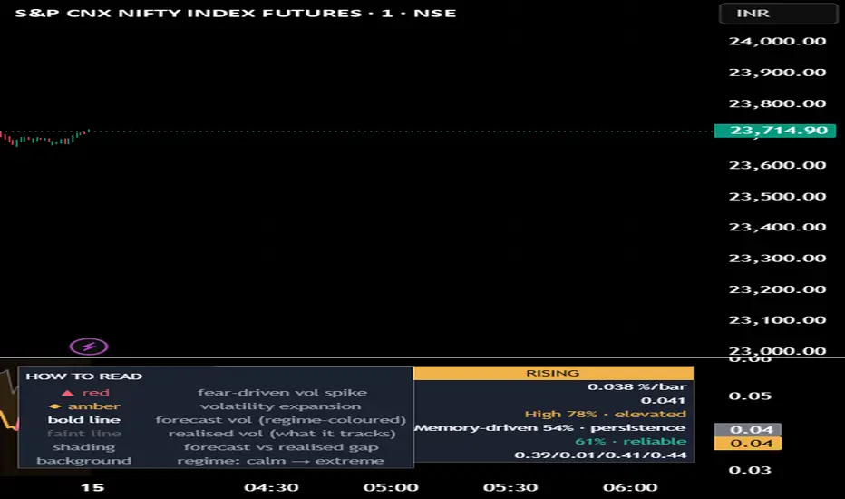
A self-calibrating forecaster of an instrument’s own **realised volatility**, built only from its price path. It estimates how large the next bar’s volatility is likely to be, explains *why* (which part of the price path is driving it), and shows *how well* that explanation is currently working on the symbol in front of you. It is **context for risk and regime awareness — not a buy/sell signal and not a strategy.** It plots in a sub-pane: a forecast line, the realised-vol line it tracks, regime shading, and a compact dashboard.
### The idea, in one paragraph
Volatility is largely **path-dependent**: an asset’s volatility is mostly explained by its own recent price path. Falling prices tend to lift volatility (the leverage effect), recent movement tends to persist (volatility clustering), and strong rallies add their own volatility. This script turns that idea into a working, per-instrument forecaster and then proves the fit on-chart.
### Why these components are combined (mashup justification)
This is **one model expressed as a single estimate → explain → calibrate → decompose → verify loop**, not a bundle of unrelated indicators stacked together. Each stage is necessary; remove any one and the result breaks:
1. **Realised-volatility estimator** (range-based Garman-Klass, or close-to-close) measures the ground-truth volatility the model is trying to explain. Without it there is nothing to fit to.
2. **Path features** are the model’s inputs: a *trend / leverage* feature (a weighted average of recent returns) and an *activity / churn* feature (the square root of a weighted average of recent squared returns), each built as a blend of fast, medium and slow kernels so it carries short **and** long memory; plus an **upside-convexity** term (so strong rallies add volatility) and a **persistence (memory)** term (a longer-horizon average of past realised vol). Features without calibration are unscaled noise.
3. **Rolling ridge calibration** fits the weights of `realised_vol ≈ b0 + b1·trend + b2·activity + b12·upside + b3·memory` to *this* instrument by rolling regression. The predictors are correlated, so the fit is **ridge-regularised on standardised predictors** to keep the coefficients steady. Calibration without features has nothing to fit; features without calibration cannot be put in the right units.
4. **Decomposition** splits the forecast into its drivers — **Path** (leverage / upside), **Activity** (churn), and **Memory** (persistence) — which is the interpretation the model makes possible.
5. **Live fit read-out** (rolling R² of forecast vs realised) is the proof the loop is working on the asset in front of you.
So the five parts are stages of a single pipeline: measure realised vol, explain it from the path, calibrate to the instrument, decompose it, and verify the fit — one engine, not five overlays.
### How it works (more detail)
- **Inputs are lagged one bar.** The path features are built from confirmed past returns, so each bar’s forecast is known before that bar’s own return forms — a genuine one-step-ahead forecast. Historical values do not change.
- **Kernels.** Each feature blends a fast, a medium and a slow-tail kernel. The slow tail approximates the heavy, slowly-decaying weighting that long-memory volatility requires; the fast kernel keeps it responsive.
- **Positivity.** The activity feature is floored to stay strictly positive, keeping the forecast well-defined.
- **Calibration.** A 4-predictor ridge regression is solved each bar over a rolling window via standardised correlation-matrix inversion, then mapped back to raw units. Ridge (a single, adjustable penalty) is what keeps the correlated predictors from producing erratic coefficients.
### How to read it
- **Bold line** = the model’s volatility **forecast**; **faint line** = the **realised** volatility it tracks. Close agreement = the model fits here.
- **Driver** tells you *why* volatility is where it is: **Path** (a falling path lifting vol = leverage/fear, or a strong rally = upside), **Activity** (recent churn persisting), or **Memory** (volatility coasting on its own persistence). The % is that channel’s share.
- **Model fit** is the rolling R² — how much of realised-vol variance the path explains on this symbol. Trust the forecast more when it is high; treat it cautiously when it reads “weak.”
- **Regime** (Low / Normal / High / Extreme) is the forecast’s own percentile. Rising vol from a Low regime is an expansion; this is context, not a trade call.
- **Markers:** ▲ red = a fear-driven spike; ◆ amber = a volatility expansion into the High regime.
A practical note: this forecasts the **size** of moves, not their **direction**. A high forecast says “expect bigger swings,” not “go long/short.” Typical uses are risk-management context (sizing, stop width), regime filtering (compressed Low regimes precede expansions; Extreme regimes tend to mean-revert), and options-style context (is volatility likely to rise or fade) — always as context layered on your own method.
### Universal data layer (works on any asset, any market)
The script reads the chart’s own symbol by default, so it runs on equities, futures, FX, crypto and indices with no configuration. Settings let you:
- choose the **price source** (close / hl2 / hlc3 / ohlc4),
- optionally compute the forecast on a **different symbol** than the one charted,
- optionally run on a **fixed calculation timeframe** for a stable basis,
- choose the realised-vol estimator (range-based or close-to-close) for symbols with or without usable ranges.
The dashboard theme is **adaptive**: it reads the chart background and keeps text and cells legible on dark or light colour schemes (or you can force Dark/Light).
### What makes it original
A working, per-instrument path-dependent **realised-volatility forecaster** with rolling ridge self-calibration, a three-way (Path / Activity / Memory) decomposition, and an on-chart fit score — a recent institutional volatility concept made legible and measurable on a chart, rather than an ATR or a standard-deviation band. It does not merely display a volatility statistic; it fits a small volatility model to the symbol and shows you both the forecast and how much to trust it.
### Limitations (honest)
- Volatility is forecastable but never certain. The realised-volatility research this builds on explains a **minority** of realised-vol variance even at its best, so a rolling fit in the 0.3–0.6 range is doing well, not failing.
- The forecast is a **reduced, practical form** of the underlying framework; it is meant as context, not a precise volatility product.
- The fit dips through structural breaks; the dashboard shows it (“weak”), which is itself useful information.
- An optional higher calculation timeframe than the chart can update intrabar until that bar closes; the default (chart timeframe) does not.
### Credits
The path-dependent volatility framework this script operationalises is from the academic work of **J. Guyon and J. Lekeufack, “Volatility is (mostly) path-dependent” (2023)**. The persistence/memory predictor follows the heterogeneous-autoregressive (HAR) realised-volatility approach of **F. Corsi (2009)**. The range-based realised-variance estimator is **Garman & Klass (1980)**. The activity-positivity treatment follows results by **Nutz & Riveros Valdevenito** and **Andrès & Jourdain**. This implementation, the rolling ridge self-calibration, the Path/Activity/Memory decomposition, and the on-chart fit score are the author’s own work.
### Disclaimer
This script is a study/indicator for chart analysis and education only. It is **not** a strategy, **not** a recommendation, and **not** financial advice. It places no orders and guarantees no outcome. All values are estimates derived from price and can be wrong, especially through structural breaks and on illiquid or low-history symbols. Markets carry risk; do your own research and manage your own risk.
### What it is
A self-calibrating forecaster of an instrument’s own **realised volatility**, built only from its price path. It estimates how large the next bar’s volatility is likely to be, explains *why* (which part of the price path is driving it), and shows *how well* that explanation is currently working on the symbol in front of you. It is **context for risk and regime awareness — not a buy/sell signal and not a strategy.** It plots in a sub-pane: a forecast line, the realised-vol line it tracks, regime shading, and a compact dashboard.
### The idea, in one paragraph
Volatility is largely **path-dependent**: an asset’s volatility is mostly explained by its own recent price path. Falling prices tend to lift volatility (the leverage effect), recent movement tends to persist (volatility clustering), and strong rallies add their own volatility. This script turns that idea into a working, per-instrument forecaster and then proves the fit on-chart.
### Why these components are combined (mashup justification)
This is **one model expressed as a single estimate → explain → calibrate → decompose → verify loop**, not a bundle of unrelated indicators stacked together. Each stage is necessary; remove any one and the result breaks:
1. **Realised-volatility estimator** (range-based Garman-Klass, or close-to-close) measures the ground-truth volatility the model is trying to explain. Without it there is nothing to fit to.
2. **Path features** are the model’s inputs: a *trend / leverage* feature (a weighted average of recent returns) and an *activity / churn* feature (the square root of a weighted average of recent squared returns), each built as a blend of fast, medium and slow kernels so it carries short **and** long memory; plus an **upside-convexity** term (so strong rallies add volatility) and a **persistence (memory)** term (a longer-horizon average of past realised vol). Features without calibration are unscaled noise.
3. **Rolling ridge calibration** fits the weights of `realised_vol ≈ b0 + b1·trend + b2·activity + b12·upside + b3·memory` to *this* instrument by rolling regression. The predictors are correlated, so the fit is **ridge-regularised on standardised predictors** to keep the coefficients steady. Calibration without features has nothing to fit; features without calibration cannot be put in the right units.
4. **Decomposition** splits the forecast into its drivers — **Path** (leverage / upside), **Activity** (churn), and **Memory** (persistence) — which is the interpretation the model makes possible.
5. **Live fit read-out** (rolling R² of forecast vs realised) is the proof the loop is working on the asset in front of you.
So the five parts are stages of a single pipeline: measure realised vol, explain it from the path, calibrate to the instrument, decompose it, and verify the fit — one engine, not five overlays.
### How it works (more detail)
- **Inputs are lagged one bar.** The path features are built from confirmed past returns, so each bar’s forecast is known before that bar’s own return forms — a genuine one-step-ahead forecast. Historical values do not change.
- **Kernels.** Each feature blends a fast, a medium and a slow-tail kernel. The slow tail approximates the heavy, slowly-decaying weighting that long-memory volatility requires; the fast kernel keeps it responsive.
- **Positivity.** The activity feature is floored to stay strictly positive, keeping the forecast well-defined.
- **Calibration.** A 4-predictor ridge regression is solved each bar over a rolling window via standardised correlation-matrix inversion, then mapped back to raw units. Ridge (a single, adjustable penalty) is what keeps the correlated predictors from producing erratic coefficients.
### How to read it
- **Bold line** = the model’s volatility **forecast**; **faint line** = the **realised** volatility it tracks. Close agreement = the model fits here.
- **Driver** tells you *why* volatility is where it is: **Path** (a falling path lifting vol = leverage/fear, or a strong rally = upside), **Activity** (recent churn persisting), or **Memory** (volatility coasting on its own persistence). The % is that channel’s share.
- **Model fit** is the rolling R² — how much of realised-vol variance the path explains on this symbol. Trust the forecast more when it is high; treat it cautiously when it reads “weak.”
- **Regime** (Low / Normal / High / Extreme) is the forecast’s own percentile. Rising vol from a Low regime is an expansion; this is context, not a trade call.
- **Markers:** ▲ red = a fear-driven spike; ◆ amber = a volatility expansion into the High regime.
A practical note: this forecasts the **size** of moves, not their **direction**. A high forecast says “expect bigger swings,” not “go long/short.” Typical uses are risk-management context (sizing, stop width), regime filtering (compressed Low regimes precede expansions; Extreme regimes tend to mean-revert), and options-style context (is volatility likely to rise or fade) — always as context layered on your own method.
### Universal data layer (works on any asset, any market)
The script reads the chart’s own symbol by default, so it runs on equities, futures, FX, crypto and indices with no configuration. Settings let you:
- choose the **price source** (close / hl2 / hlc3 / ohlc4),
- optionally compute the forecast on a **different symbol** than the one charted,
- optionally run on a **fixed calculation timeframe** for a stable basis,
- choose the realised-vol estimator (range-based or close-to-close) for symbols with or without usable ranges.
The dashboard theme is **adaptive**: it reads the chart background and keeps text and cells legible on dark or light colour schemes (or you can force Dark/Light).
### What makes it original
A working, per-instrument path-dependent **realised-volatility forecaster** with rolling ridge self-calibration, a three-way (Path / Activity / Memory) decomposition, and an on-chart fit score — a recent institutional volatility concept made legible and measurable on a chart, rather than an ATR or a standard-deviation band. It does not merely display a volatility statistic; it fits a small volatility model to the symbol and shows you both the forecast and how much to trust it.
### Limitations (honest)
- Volatility is forecastable but never certain. The realised-volatility research this builds on explains a **minority** of realised-vol variance even at its best, so a rolling fit in the 0.3–0.6 range is doing well, not failing.
- The forecast is a **reduced, practical form** of the underlying framework; it is meant as context, not a precise volatility product.
- The fit dips through structural breaks; the dashboard shows it (“weak”), which is itself useful information.
- An optional higher calculation timeframe than the chart can update intrabar until that bar closes; the default (chart timeframe) does not.
### Credits
The path-dependent volatility framework this script operationalises is from the academic work of **J. Guyon and J. Lekeufack, “Volatility is (mostly) path-dependent” (2023)**. The persistence/memory predictor follows the heterogeneous-autoregressive (HAR) realised-volatility approach of **F. Corsi (2009)**. The range-based realised-variance estimator is **Garman & Klass (1980)**. The activity-positivity treatment follows results by **Nutz & Riveros Valdevenito** and **Andrès & Jourdain**. This implementation, the rolling ridge self-calibration, the Path/Activity/Memory decomposition, and the on-chart fit score are the author’s own work.
### Disclaimer
This script is a study/indicator for chart analysis and education only. It is **not** a strategy, **not** a recommendation, and **not** financial advice. It places no orders and guarantees no outcome. All values are estimates derived from price and can be wrong, especially through structural breaks and on illiquid or low-history symbols. Markets carry risk; do your own research and manage your own risk.
Скрипт с открытым кодом
В истинном духе TradingView, создатель этого скрипта сделал его открытым исходным кодом, чтобы трейдеры могли проверить и убедиться в его функциональности. Браво автору! Вы можете использовать его бесплатно, но помните, что перепубликация кода подчиняется нашим Правилам поведения.

Отказ от ответственности
Информация и публикации не предназначены для предоставления и не являются финансовыми, инвестиционными, торговыми или другими видами советов или рекомендаций, предоставленных или одобренных TradingView. Подробнее читайте в Условиях использования.
Скрипт с открытым кодом
В истинном духе TradingView, создатель этого скрипта сделал его открытым исходным кодом, чтобы трейдеры могли проверить и убедиться в его функциональности. Браво автору! Вы можете использовать его бесплатно, но помните, что перепубликация кода подчиняется нашим Правилам поведения.
Отказ от ответственности
Информация и публикации не предназначены для предоставления и не являются финансовыми, инвестиционными, торговыми или другими видами советов или рекомендаций, предоставленных или одобренных TradingView. Подробнее читайте в Условиях использования.