[Suitable Hope] Crypto Upside Model 3.0The "Crypto Upside Model 3.0" indicator dynamically calculates the potential price of any cryptocurrency based on various percentages of Ethereum or Bitcoin's market capitalization.
By fetching and analyzing marketcap data from TradingView sources, it allows traders to visualize potential price targets if their chosen cryptocurrency reaches specific market dominance levels. This tool is designed for daily timeframe analysis and can be used to set informed price expectations and strategic investment goals, providing valuable insights for long-term investment planning.
Why using the Crypto Upside Model 3.0?
Strategic Planning: Helps traders and investors set realistic price targets and investment goals by visualizing potential market cap scenarios.
Informed Decision-Making: Provides a data-driven approach to understanding how a cryptocurrency might perform relative to major assets like Bitcoin and Ethereum.
Customizable Analysis: Allows users to choose different comparison assets (ETH or BTC) and visualize various market cap dominance percentages, offering tailored insights.
Daily Timeframe Focus: Ideal for swing traders and long-term investors who operate on a daily analysis timeframe, providing relevant and actionable data.
Bull Markets: Identify potential price targets if your cryptocurrency's market cap increases significantly.
Bear Markets: Assess how much value could be retained relative to major cryptocurrencies.
Strategic Entry/Exit Points: Use the visualized targets to plan entry or exit points in your trading strategy.
Comparative Advantage
Dynamic Adaptation: Unlike fixed indicators, this tool adapts to any active chart, making it versatile for multiple cryptocurrencies.
Market Cap Insights: Provides a unique perspective by linking price targets to market cap dominance, a critical factor in the crypto market.
User Instructions
Setup: Add the " Upside Model 3.0" indicator to your TradingView chart.
Configuration: Use the input settings to select the comparison cryptocurrency (ETH or BTC) and enable the desired market cap percentage plots.
Analysis: The indicator will display potential price targets based on the selected market cap percentages, providing a visual guide for setting price expectations.
Limitations
Marketcap Data Availability: The indicator relies on marketcap data from TradingView, which may not be available for all cryptocurrencies. If the data is unavailable, the indicator will not function for that asset. This tool is more likely to work with older, established cryptocurrencies, as marketcap data for newer cryptocurrencies may not yet be available.
Daily Timeframe Restriction: The indicator is designed to work exclusively on the daily timeframe, limiting its applicability for intraday trading.
Assumptions of Market Dynamics: The calculations assume a direct correlation between market dominance and price, which may not account for other market dynamics and external factors influencing prices.
Data Accuracy: The accuracy of the indicator depends on the reliability of the data provided by TradingView, which may sometimes experience delays or inaccuracies.
Currently available cryptocurrencies: Bitcoin, Ethereum, Solana, Binance Coin, Cardano, Ripple, Polkadot, Avalanche, Chainlink, Litecoin, Dogecoin, Terra, Uniswap, VeChain, Stellar, Internet Computer, Hedera, Filecoin, Monero, Aave, TRON, NEAR Protocol, Compound, Maker,... For all compatible cryptocurrencies, please consult CRYPTOCAP's documentation.
Final notes
Although various sources ask a payment or user data for similar kind of private indicators, this one is entirely free and open source. "Uncanny" isn't it? I hope this indicator will provide you value. Feel free to leave a message if you have any questions or constructive feedback.
Examples of how I use this indicator
When using ETH's historical price as a reference compared to Bitcoin's marketcap, we can notice that price generally has been held between the +-30% and 50% lines of BTC's marketcap. If history is repeating again, we can expect major resistances around the 50% looking ahead into the future. This for me would be a great area to potentially reduce my ETH spot position.
When using SOL's historical price action, we can notice that the 15% line of ETH's marketcap has been a top in the previous cycle. Today SOL (July 2024), is back at this level. Could this be a top again or could price break this 15% level and head perhaps towards 30% which currently sits around $260? Time will tell.
These are 2 simple example of how I interpret the data. I'm keen to hear what other findings with other pairs you can find. Индикатор

Стратегия
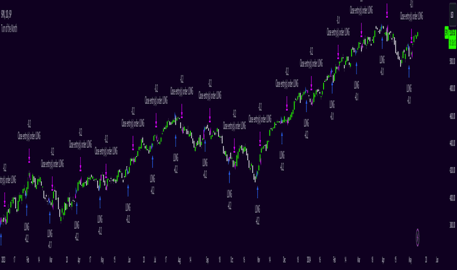
Index investingThe Index Investing indicator simplifies decision-making for adding to Index ETF's Long-term investments. By utilizing a percentage discount methodology, it highlights potential opportunities to enhance portfolios. This straightforward tool aids in identifying favorable moments to invest based on calculated price discounts from selected reference points, making the process more systematic and less subjective.
🔶 SETTINGS
Reference Price: Choose between 'All-Time-High' or 'Start of the Year' as the basis for calculating discount levels. This allows for flexibility in strategy depending on market conditions or investment philosophy.
Discount 1 %, Discount 2 %, Discount 3 %: These inputs define the percentage below the reference price at which buy signals are generated. They represent strategic entry points at discounted prices.
🔶 Default Parameters
The default parameters of 4.13%, 8.26%, and 12.39% for the discount levels are chosen based on the average 5-year return of the NSE:NIFTY Index, which stands at approximately 12.39%. By dividing this return into three parts, we obtain a structured approach to capturing potential upside at varying levels of market retracement, providing a logical basis for the selected default values.
Users have the flexibility to modify these parameters, tailoring the indicator to fit their unique approach and market outlook.
🔶 How Levels Are Calculated
Discount levels are calculated using the formula: Discount Price = Reference Price * (1 - Discount %) . This succinct approach establishes specific entry points below the chosen reference, such as an all-time high or the year's start price.
🔶 How Are the Buy Labels Generated
Buy signals are generated when the market price(Low of the candle) crosses under any of the defined discount levels. Each level has a corresponding buy label ('Buy 1', 'Buy 2', 'Buy 3'), which is activated upon the price crossing below the specified discount level and is only reset at the beginning of a new year or upon reaching a new reference high, ensuring signals are not repetitive for the same price level.
🔶 Other Features
Alerts: The indicator provides alerts for each buy signal, notifying potential entry points at their defined discount levels. The alert triggers only once per candle.
Year Marker: A vertical line with an accompanying label marks the start of each trading year on the chart. This feature aids in visualizing the temporal context of buy signals and reference price adjustments.
Индикатор

RSI Volatility Bands [QuantraSystems]RSI Volatility Bands
Introduction
The RSI Volatility Bands indicator introduces a unique approach to market analysis by combining the traditional Relative Strength Index (RSI) with dynamic, volatility adjusted deviation bands. It is designed to provide a highly customizable method of trend analysis, enabling investors to analyze potential entry and exit points in a new and profound way.
The deviation bands are calculated and drawn in a manner which allows investors to view them as areas of dynamic support and resistance.
Legend
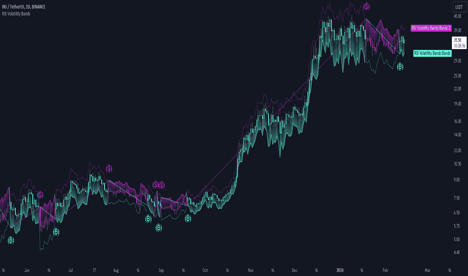
Upper and Lower Bands - A dynamic plot of the volatility-adjusted range around the current price.
Signals - Generated when the RSI volatility bands indicate a trend shift.
Case Study
The chart highlights the occurrence of false signals, emphasizing the need for caution when the bands are contracted and market volatility is low.
Juxtaposing this, during volatile market phases as shown, the indicator can effectively adapt to strong trends. This keeps an investor in a position even through a minor drawdown in order to exploit the entire price movement.
Recommended Settings
The RSI Volatility Bands are highly customisable and can be adapted to many assets with diverse behaviors.
The calibrations used in the above screenshots are as follows:
Source = close
RSI Length = 8
RSI Smoothing MA = DEMA
Bandwidth Type = DEMA
Bandwidth Length = 24
Bandwidth Smooth = 25
Methodology
The indicator first calculates the RSI of the price data, and applies a custom moving average.
The deviation bands are then calculated based upon the absolute difference between the RSI and its moving average - providing a unique volatility insight.
The deviation bands are then adjusted with another smoothing function, providing clear visuals of the RSI’s trend within a volatility-adjusted context.
rsiVal = ta.rsi(close, rsiLength)
rsiEma = ma(rsiMA, rsiVal, bandLength)
bandwidth = ma(bandMA, math.abs(rsiVal - rsiEma), bandLength)
upperBand = ma(bandMA, rsiEma + bandwidth, smooth)
lowerBand = ma(bandMA, rsiEma - bandwidth, smooth)
long = upperBand > 50 and not (lowerBand < lowerBand and lowerBand < 50)
short= not (upperBand > 50 and not (lowerBand < lowerBand and lowerBand < 50))
By dynamically adjusting to market conditions, the RSI trend bands offer a unique perspective on market trends, and reversal zones.
Индикатор
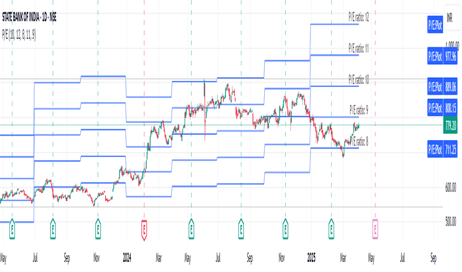
EPS GridIntroduction:
This simple indicator offers insights into the relationship between stock prices and earnings, aiding in the assessment of valuation dynamics during different periods.
Understanding Price-to-Earnings (P/E) Ratio:
The commonly used Price to Earnings (P/E) ratio, calculated as Current Price divided by Earnings Per Share (EPS) over the trailing 12 months (TTM), serves as a fundamental metric. Here, we use this formula to estimate a stock's price. For instance, multiplying EPS by 10 provides an approximation of the stock price with a P/E ratio of 10.
The Grid Concept:
Utilizing this principle, a visual grid is constructed to illustrate how stock prices correlate with earnings. This grid facilitates the identification of both potential bargains and overvalued stocks.
How to Utilize:
This indicator is pre-configured with earnings multiples of 10, 15, 20, and 25. Simply add it to your chart and observe whether earnings demonstrate consistent growth. If prices lag behind earnings, a potential catch-up phase may ensue in the future.
Happy Investing!
Embark on your investment journey armed with this indicator, and may it guide you towards informed decisions and successful ventures. Индикатор
Simple Neural Network Transformed RSI [QuantraSystems]Simple Neural Network Transformed RSI
Introduction
The Simple Neural Network Transformed RSI (ɴɴᴛ ʀsɪ) stands out as a formidable tool for traders who specialize in lower timeframe trading.
It is an innovative enhancement of the traditional RSI readings with simple neural network smoothing techniques.
This unique blend results in fairly accurate signals, tailored for swift market movements. The ɴɴᴛ ʀsɪ is particularly resistant to the usual market noise found in lower timeframes, ensuring a clearer view of short-term trends.
Furthermore, its diverse range of visualization options adds versatility, making it a valuable tool for traders seeking to capitalize on short-duration market dynamics.
Legend
In the Image you can see the BTCUSD 1D Chart with the ɴɴᴛ ʀsɪ in Trend Following Mode to display the current trend. This is visualized with the barcoloring.
Its Overbought and Oversold zones start at 50% and end at 100% of the selected Standard Deviation (default σ = 2), which can indicate extremely rare situations which can lead to either a softening momentum in the trend or even a mean reversion situation.
Here you can also see the original Indicator line and the Heikin Ashi transformed Indicator bars - more on that now.
Notes
Quantra Standard Value Contents:
To draw out all the information from the indicator calculation we have added a Heikin-Ashi (HA) Candle Visualization.
This HA transformation smoothens out the indicator values and gives a more informative look into Momentum and Trend of the Indicator itself.
This allows early entries and exits by observing the HA transformed Indicator values.
To diversify, different visualization options are available, either a classic line, HA transformed or Hybrid, which contains both of the previous.
To make Quantra's Indicators as useful and versatile as possible we have created options
to change the barcoloring and thus the derived signal from the indicator based on different modes.
Option to choose different Modes:
Trend Following (Indicator above mid line counts as uptrend, below is downtrend)
Extremities (Everything going beyond the Deviation Bands in a Mean Reversion manner is highlighted)
Candles (Color of HA candles as barcolor)
Reversion (HA ONLY) (Reversion Signals via the triangles if HA candles change state outside of the Deviation Bands)
- Reversion Signals are indicated by the triangles in the Heikin-Ashi or Hybrid visualization when the HA Candles revert
from downwards to upwards or the other way around OUTSIDE of the SD Bands.
Depending on the Indicator they signal OB/OS areas and can either work as high probability entries and exits for Mean Reversion trades or
indicate Momentum slow downs and potential ranges.
Please use another indicator to confirm this.
Case Study
To effectively utilize the NNT-RSI, traders should know their style and familiarize themselves with the available options.
As stated above, you have multiple modes available that you can combine as you need and see fit.
In the given example mostly only the mode was used in an isolated fashion.
Trend Following:
Purely relied on State Change - Midline crossover
Could be combined with Momentum or Reversion analysis for better entries/exits.
Extremities:
Ideal entry/exit is in the accordingly colored OS/OB Area, the Reversion signaled the latest possible entry/exit.
HA Candles:
Specifically applicable for strong trends. Powerful and fast tool.
Can whip if used as sole condition.
Reversions:
Shows the single entry and exit bars which have a positive expected value outcome.
Can also be used as confirmation or as last signal.
Please note that we always advise to find more confluence by additional indicators.
Traders are encouraged to test and determine the most suitable settings for their specific trading strategies and timeframes.
In the showcased trades the default settings were used.
Methodology
The Simple Neural Network Transformed RSI uses a simple neural network logic to process RSI values, smoothing them for more accurate trend analysis.
This is achieved through a linear combination of RSI values over a specified input length, weighted evenly to produce a neural network output.
// Simple neural network logic (linear combination with weighted aggregation)
var float inputs = array.new_float(nnLength, na)
for i = 0 to nnLength - 1
array.set(inputs, i, rsi1 )
nnOutput = 0.0
for i = 0 to nnLength - 1
nnOutput := nnOutput + array.get(inputs, i) * (1 / nnLength)
nnOutput
This output is then compared against a standard or dynamic mean line to generate trend following signals.
Mean = ta.sma(nnOutput, sdLook)
cross = useMean? 50 : Mean
The indicator also incorporates Heikin Ashi candlestick calculations to provide additional insights into market dynamics, such as trend strength and potential reversals.
// Calculate Heikin Ashi representation
ha = ha(
na(nnOutput ) ? nnOutput : nnOutput ,
math.max(nnOutput, nnOutput ),
math.min(nnOutput, nnOutput ),
nnOutput)
Standard deviation bands are used to create dynamic overbought and oversold zones, further enhancing the tool's analytical capabilities.
// Calculate Dynamic OB/OS Zones
stdv_bands(_src, _length, _mult) =>
float basis = ta.sma(_src, _length)
float dev = _mult * ta.stdev(_src, _length)
= stdv_bands(nnOutput, sdLook,sdMult/2)
= stdv_bands(nnOutput, sdLook, sdMult)
The Standard Deviation bands take defined parameters from the user, in this case sigma of ideally between 2 to 3,
to help the indicator detect extremely improbable conditions and thus take an inversely probable signal from it to forward to the user.
The parameter settings and also the visualizations allow for ample customizations by the trader.
For questions or recommendations, please feel free to seek contact in the comments.
Индикатор

Индикатор

Triple Confirmation Kernel Regression Base [QuantraSystems]Kernel Regression Oscillator - BASE
Introduction
The Kernel Regression Oscillator (ᏦᏒᎧ) represents an advanced tool for traders looking to capitalize on market trends.
This Indicator is valuable in identifying and confirming trend directions, as well as probabilistic and dynamic oversold and overbought zones.
It achieves this through a unique composite approach using three distinct Kernel Regressions combined in an Oscillator. The additional Chart Overlay Indicator adds confidence to the signal.
This methodology helps the trader to significantly reduce false signals and offers a more reliable indication of market movements than more widely used indicators can.
Legend
The upper section is the Overlay. It features the Signal Wave to display the current trend.
Its Overbought and Oversold zones start at 50% and end at 100% of the selected Standard Deviation (default σ = 3), which can indicate extremely rare situations which can lead to either a softening momentum in the trend or even a mean reversion situation.
The lower one is the Base Chart - This Indicator.
It features the Kernel Regression Oscillator to display a composite of three distinct regressions, also displaying current trend.
Its Overbought and Oversold zones start at 50% and end at 100% of the selected Standard Deviation (default σ = 2), which can indicate extremely rare situations.
Case Study
To effectively utilize the ᏦᏒᎧ, traders should use both the additional Overlay and the Base
Chart at the same time. Then focus on capturing the confluence in signals, for example:
If the 𝓢𝓲𝓰𝓷𝓪𝓵 𝓦𝓪𝓿𝓮 on the Overlay and the ᏦᏒᎧ on the Base Chart both reside near the extreme of an Oversold zone the probability is higher than normal that momentum in trend may soften or the token may even experience a reversion soon.
If a bar is characterized by an Oversold Shading in both the Overlay and the Base Chart, then the probability is very high to experience a reversion soon.
In this case the trader may want to look for appropriate entries into a long position, as displayed here.
If a bar is characterized by an Overbought Shading in either Overlay or Base Chart, then the probability is high for momentum weakening or a mean reversion.
In this case the trade may have taken profit and closed his long position, as displayed here.
Please note that we always advise to find more confluence by additional indicators.
Recommended Settings
Swing Trading (1D chart)
Overlay
Bandwith: 45
Width: 2
SD Lookback: 150
SD Multiplier: 2
Base Chart
Bandwith: 45
SD Lookback: 150
SD Multiplier: 2
Fast-paced, Scalping (4min chart)
Overlay
Bandwith: 75
Width: 2
SD Lookback: 150
SD Multiplier: 3
Base Chart
Bandwith: 45
SD Lookback: 150
SD Multiplier: 2
Notes
The Kernel Regression Oscillator on the Base Chart is also sensitive to divergences if that is something you are keen on using.
For maximum confluence, it is recommended to use the indicator both as a chart overlay and in its Base Chart.
Please pay attention to shaded areas with Standard Deviation settings of 2 or 3 at their outer borders, and consider action only with high confidence when both parts of the indicator align on the same signal.
This tool shows its best performance on timeframes lower than 4 hours.
Traders are encouraged to test and determine the most suitable settings for their specific trading strategies and timeframes.
The trend following functionality is indicated through the "𝓢𝓲𝓰𝓷𝓪𝓵 𝓦𝓪𝓿𝓮" Line, with optional "Up" and "Down" arrows to denote trend directions only (toggle “Show Trend Signals”).
Methodology
The Kernel Regression Oscillator takes three distinct kernel regression functions,
used at similar weight, in order to calculate a balanced and smooth composite of the regressions. Part of it are:
The Epanechnikov Kernel Regression: Known for its efficiency in smoothing data by assigning less weight to data points further away from the target point than closer data points, effectively reducing variance.
The Wave Kernel Regression: Similarly assigning weight to the data points based on distance, it captures repetitive and thus wave-like patterns within the data to smoothen out and reduce the effect of underlying cyclical trends.
The Logistic Kernel Regression: This uses the logistic function in order to assign weights by probability distribution on the distance between data points and target points. It thus avoids both bias and variance to a certain level.
kernel(source, bandwidth, kernel_type) =>
switch kernel_type
"Epanechnikov" => math.abs(source) <= 1 ? 0.75 * (1 - math.pow(source, 2)) : 0.0
"Logistic" => 1/math.exp(source + 2 + math.exp(-source))
"Wave" => math.abs(source) <= 1 ? (1 - math.abs(source)) * math.cos(math.pi * source) : 0.
kernelRegression(src, bandwidth, kernel_type) =>
sumWeightedY = 0.
sumKernels = 0.
for i = 0 to bandwidth - 1
base = i*i/math.pow(bandwidth, 2)
kernel = kernel(base, 1, kernel_type)
sumWeightedY += kernel * src
sumKernels += kernel
(src - sumWeightedY/sumKernels)/src
// Triple Confirmations
Ep = kernelRegression(source, bandwidth, 'Epanechnikov' )
Lo = kernelRegression(source, bandwidth, 'Logistic' )
Wa = kernelRegression(source, bandwidth, 'Wave' )
By combining these regressions in an unbiased average, we follow our principle of achieving confluence for a signal or a decision, by stacking several edges to increase the probability that we are correct.
// Average
AV = math.avg(Ep, Lo, Wa)
The Standard Deviation bands take defined parameters from the user, in this case sigma of ideally between 2 to 3,
to help the indicator detect extremely improbable conditions and thus take an inversely probable signal from it to forward to the user.
The parameter settings and also the visualizations allow for ample customizations by the trader. The indicator comes with default and recommended settings.
For questions or recommendations, please feel free to seek contact in the comments. Индикатор

White NoiseThe "White Noise" indicator is designed to visualize the dispersion of price movements around a moving average, providing insights into market noise and potential trend changes. It highlights periods of increased volatility or noise compared to the underlying trend.
Code Explanation:
Inputs:
mlen: Input for the length of the noise calculation.
hlen: Input for the length of the Hull moving average.
col_up: Input for the color of the up movement.
col_dn: Input for the color of the down movement.
Calculations:
ma: Calculate the simple moving average of the high, low, and close prices (hlc3) over the specified mlen period.
dist: Calculate the percentage distance between the hlc3 and the moving average ma, then scale it by 850. This quantifies the deviation from the moving average as a value.
sm: Smooth the calculated dist values using a weighted moving average (WMA) twice, with different weights, and subtract one from the other. This provides a smoothed representation of the dispersion.
Coloring:
col_wn: Determine the color of the bars based on whether dist is positive or negative and whether it's greater or less than the smoothed sm value. This creates color-coded columns indicating upward or downward movements with varying opacity.
col_switch: Define the color for the current trend state. It switches color when the smoothed sm crosses above or below its previous value, indicating potential trend changes.
col_switch2: Define the color for the horizontal line that separates the two trend states. It switches color based on the same crossover and crossunder conditions as col_switch.
Plots:
plot(dist): Plot the dispersion values as columns with color defined by col_wn.
plot(sm): Plot the smoothed dispersion line with a white color and thicker linewidth.
plot(sm ): Plot the previous smoothed dispersion value with a lighter white color to create a visual distinction.
Usage:
This indicator can help traders identify periods of increased market noise, visualize potential trend reversals, and assess the strength of price movements around the moving average. The colored columns and smoothed line offer insights into the ebb and flow of market sentiment, aiding in decision-making.
ps. This can be used as a long-term TPI component if you dabble in Modern Portfolio Theory (MPT)
Recommended for timeframes on the 1D or above:
Индикатор

Индикатор

Индикатор

Стратегия

Индикатор

Индикатор
Стратегия

Индикатор

Стратегия

Nico's SPX Dynamic ChannelsTest of dynamic channels and some statistics made by hand.
This indicator was done specifically for the S&P500 index.
As you can see, below the 125 EMA there's a lot more volatility than in the upside. I've made some kind of a dynamic linear regression of the lows and the highs.
I've chosen the MA that best fits the SPX, and then calculated in Excel the percental mean and SDs of most important peaks and valleys that I've chosen in comparison to the 125 MA. This lead to the green, orange and red zones. BUT, I've calculated the peaks and valleys separately, as I assumed that a bear market and crashes have way more volatility than bull markets. That's why the difference between the upper and the lower channels.
The neutral blue zone is composed by an upper EMA of the highs and lower EMA of the lows. No MA in this script uses the close price as a source.
This MA makes sense because it represents a semester of trading, for this particular asset.
Backtest results
It's also interesting to try it here too, as it has a little bit more of data:
SPCFD:SPX
As it's not a trading system, I have no batting average nor ratios for this.
Still, the measures of the peaks and valleys are very accurate and repeat themselves over and over again. The results were:
3rd resistance: 12.88%
2nd resistance: 10.12%
1st resistance: 7.36%
1st support: -6.42%
2nd support: -14.8%
3rd support: -23.18%
All referred to the mean, which is the 125 EMA zone.
After the 1950's works like magic, but not before. You will see that it doesn't work in the great depression and it's crash.
How to use this indicator
Green = First grade support/resistance .
Orange = Second grade support/resistance . Caution.
Red = Third grade support/resistance . High chances of mean reversal.
Blue zone = This is the neutral zone, where the prices are not cheap nor expensive.
Often in a trending market, the price will have the blue zone as it's main support and when trending the price will stick to the green MA.
When the price touches the orange MA, the most probable is that it will return to the green MA.
If the price touches the red zone, there's a high chance that this is a big turning point and it will reverse to the mean (green or blue zone).
Imagine you've bought each time the price touched the red support, check that and you'll start liking this indicator. I think it is a great entry point for investors. The red resistance is good too, but of course it works for a short period of time.
I've backtested this indicator since the beginning of the dataset and it works like magic, but ONLY for the SPX index (spot price).
Leave a comment or some coins if you like it!!!
(I've posted it before like an analysis, not as a script, my bad) Индикатор

Long RSIThe RSI is a technical indicator generally used with the general setting being 14 days, and often shorter.
The accepted view is that a level of 70 indicates overbought conditions, and 30 indicates oversold conditions.
A short RSI setting will give signals quite often, and they might sometimes contradict each other.
As a individual investor, perhaps with a background in fundamental analysis, the RSI might be overlooked for other fundamental metrics.
But the idea here is that longer RSI settings can be used for investing.
The problem that arises is how to know when the indicator has reached a level that is either overbought or oversold.
This script solves that by using a specific look back period (selectable, but the standard is 1 year), and plotting the highest/lowest value that the RSI has had for that time period.
The idea is that a buy signal occurs when the indicator is at a 'historic' low, and a sell signal occurs when it at its 'historic' high.
Since you generally want to buy when the indicator is at its low, and has stopped decreasing, the script comes with a function that shows you when yesterdays value reached a historic low, but todays value is higher than yesterday.
This is shown by a color change of the background to green. The same is true, but opposite, for sell signals and then the background turns red.
THIS IS NOT TRADING ADVICE, AND YOU SHOULD ALWAYS DO YOUR OWN RESEARCH
GOOD LUCK AND HAPPY TRADING Индикатор

Стратегия

Индикатор

Стратегия