TURKS - Tiered Unit Risk Kernel StrategyTURKS decides how much of a long position to hold. Exposure is a graded function of where the close sits against four moving averages (20/50/100/200), so it moves in rungs rather than switching on and off. That function is monotone in price, which means it inverts: every rung has exactly one price. The panel prints those prices before they are reached — a ladder of levels at which the position gets larger or smaller, readable today.
Long-only, 0 to 1, no shorting and no leverage.
📊 THE RESULT
Twelve symbols, shipped defaults, 4-hour charts, full available history. Commission $1.50 per order, slippage 0.01xATR per side, idle cash credited nothing. b&h is buy-and-hold over the identical bars, charged nothing at all. The comparison is deliberately rigged against the strategy.
CAGR MAX DRAWDOWN CAGR / maxDD
symbol sample TURKS b&h TURKS b&h TURKS b&h
SNDK 1.3y +1406.3% +1899.0% -37.2% -56.8% 37.82 33.43
ETH 9.5y +117.3% +71.9% -54.4% -94.1% 2.16 0.76
BTC 9.5y +70.0% +54.2% -62.3% -83.9% 1.12 0.65
ARM 2.7y +62.5% +72.9% -39.8% -55.8% 1.57 1.31
TSLA 15.9y +32.7% +41.7% -57.0% -74.9% 0.57 0.56
NVDA 22.4y +25.3% +36.4% -77.0% -85.2% 0.33 0.43
AMD 21.4y +20.2% +17.3% -69.3% -96.1% 0.29 0.18
AVGO 16.8y +16.9% +39.0% -36.9% -50.3% 0.46 0.78
MU 22.4y +9.3% +19.7% -81.4% -90.9% 0.11 0.22
GOLD 13.5y +7.2% +7.7% -20.0% -35.0% 0.36 0.22
SPY 20.4y +4.4% +9.1% -40.5% -56.7% 0.11 0.16
INTC 20.4y +2.2% +8.5% -73.3% -74.2% 0.03 0.11
CAGR / maxDD is the column that settles it — return earned per unit of drawdown suffered. On that measure TURKS wins on 7 of 12. It cut maximum drawdown on 12 of 12, and beat buy-and-hold on raw return on 3.
▸ ETH — 117.3% against 71.9%, at −54.4% drawdown against −94.1%. Nearly double the return on barely half the pain.
▸ BTC — 70.0% against 54.2%, at −62.3% against −83.9%.
▸ AMD — 20.2% against 17.3%, turning a −96.1% hole into −69.3% across 21.4 years.
These are assets that spent their entire sample inside a historic bull market, measured against a benchmark paying no commission and no slippage. Halving a drawdown is ordinary. Halving it and finishing ahead is not.
BTCUSD 4h at the shipped defaults. The ladder is the green and red boxes; the envelope is the pair of curves around the mean. Bottom left is the BOOK panel reading 70.0% against 54.2% buy-and-hold at −62.3% drawdown against −83.9%, on 58.0% average exposure. Right side is the live state: what the rule targets now, where the next rung sells, where it buys back.
MU, SPY, TSLA and INTC are in that table because they were chosen to be difficult, and they behave exactly as the mechanism predicts. The rule sells strength and holds cash: it pays when a price path is violent relative to its drift, and it costs when the drift is high and the path is smooth. On a broad index it is the wrong tool — SPY 9.1% becomes 4.4%, and that number is in the table rather than left out of it.
📖 HOW TO USE IT
1 — Set your costs before you read anything. Commission ($ per order) and Typical position size ($) are the only two numbers the cost model needs; every other cost figure is a rate derived from them. A flat $1.50 is 1.9bp on an $8,000 position and 7.5bp on a $2,000 one. Leave these wrong and the panel lies to you.
2 — Pick the instrument. Single names and crypto whose drawdowns are violent relative to their drift. The table above is the guide, including the four rows that say don't.
3 — Read the ladder, not the arrows. The SELL / BUY ENGINE block prints three live numbers:
▸ Sell next above — the price at which the next rung comes off
▸ Buy back below — the price at which it goes back on
▸ Rungs sold — how much the envelope has already taken off, e.g. 12 of 20
Both prices exist now, before the move. They are not marks that appeared after one.
4 — Read the dial. The THE RULE block prints Target weight, which is what the rule says you should be holding at this instant, and Dial c / f. The POSITION block prints what you actually hold, your entry, your open return, and the round-trip cost you are currently carrying — so the gap between intention and position is always visible.
5 — Size it with c and f, not by fighting the rungs. c scales the whole position down. f is the floor you keep while the rule is off; raising it walks the book continuously toward buy-and-hold. Both tooltips print the measured frontier — the whole curve of what each step costs in return and buys in drawdown, including the region where the rule loses to simply holding less.
6 — Verify on your own symbol before trusting any of this. The BOOK panel prints Sample, CAGR against b&h, Max drawdown against b&h, CAGR/maxDD, Sharpe, Exposure and Turnover for whatever chart you are on, net of your own cost settings. Change the symbol and the whole table above regenerates for your instrument in one bar.
7 — Alerts. alert() messages ship on; JSON webhook format is a checkbox away.
🪜 HOW THE EXPOSURE IS SET
Exposure Shape picks the weighting rule. Ensemble 20/50/100/200 (graded) is the default: a slice is sold as the close drops below one more mean, bought back the same way, flat only below all four. Graded (continuous) uses one mean with an ATR ramp. Binary gate (legacy) is the original all-or-nothing rule.
Risk dial c scales the entire position down. Risk dial f is how much you keep while the rule is off. These two are the real levers, and nothing about their trade-off is hidden behind a paywall or a marketing claim — the full measured frontier is printed in the settings dialog.
Quantise Steps rounds the target to N reachable weights and requires price to clear 75% of a step before acting, so orders do not fire every bar. Ramp Width (xATR) sets how far above the mean price must travel to earn full size.
✂️ THE NADARAYA-WATSON SELL ENGINE
A trend weight cuts into weakness by construction, so it sells low: 59% of every unit the dial sells goes out below its own average cost, at 12.4 round trips a year. That is the flaw this block exists to fix. It replaces or constrains the sell side with a Gaussian kernel-regression envelope that only sells into genuine extension.
Sell Engine Mode — Dial, NWE-gated (default) keeps the dial's targets but forbids cutting while price sits below the smoother; it may still add. NWE band only turns the dial's sells off entirely. Dial + NWE (both cut) lets either one sell. Dial only leaves the envelope drawn but inert.
Sell Rungs is how much leaves on each upper-band cross: 1/N of the position. Going from 3 to 10 halved turnover, cut the share sold below basis from 16.7% to 8.9%, and pulled out-of-sample drawdown from −32.6% to −18.3%. It ships at 20, one step further along the same gradient; 10 is the last value with a formal table behind it.
Band Multiplier (3.0) and Buy-back Multiplier (2.5) set the upper and lower halfwidths in mean-absolute-deviation units. The asymmetry is the point: buying back nearer the mean than you sold restores the position before price has fully round-tripped, which is what keeps the overlay from bleeding in a chop. Bandwidth h widens and slows the smoother; it ships at 5.
🔬 HOW THIS WAS BUILT
Nine candidate signal families were tested against a matched-exposure control across 140 markets and 8,793 sessions: moving-average and momentum structure, cross-sectional relative strength, short-horizon mean reversion, volatility-of-volatility and regime transitions, drawdown state, volume, range compression, multi-timeframe agreement, and calendar seasonality. Not one was positive both in and out of sample. All nine were deleted from the codebase rather than left in as decoration.
The cleanest demonstration: take the original engine's own weight path and fire it 60 trading days late — same trades, same sizes, same turnover, same average exposure, only the dates broken. It scores better late than on time. Block-shuffling the path also beats it. A rule whose dates carry information cannot survive having them destroyed, so that engine was removed and what remains is geometry.
The stretch-proportional alternative to fixed rungs was then built and measured across 44 configurations. None beat rungs = 10. The project's pre-registered five-clause acceptance test passed all 20 graded cells — but a constant weight of 1.0 also passes three of five clauses, exactly one cell of twenty reaches p < 0.05 uncorrected (the null expectation for twenty tests), that p fails Bonferroni, and the cells are 0.985-correlated. It was reported as a failed test.
Everything left in this script survived a process designed to kill it. What remains is a sizing rule with no forecast in it: it does not predict the retest, it tells you at a price you can read now exactly what happens when one arrives.
⚙️ COSTS, AND THE SETTINGS THAT DECIDE THEM
Initial capital 150,000; commission $1.50 cash per order; no pyramiding; orders processed on bar close. Sell Engine Mode Dial, NWE-gated, Exposure Shape Ensemble 20/50/100/200 (graded), c = 1.00, f = 0.00, Quantise Steps 3, Ramp 1.0 ATR, Trend Mean 200, Cash Yield 0.00%. Envelope: bandwidth 5, multiplier 3.0, buy-back 2.5, MAE window 499, Sell Rungs 20.
TradingView's strategy() slippage is denominated in ticks, and a tick is an absolute price — one tick cannot be simultaneously correct for a $20 stock and a $1,600 one, nor for the same stock at $0.21 and at $224. It is therefore left at 0, and a proportional Slippage (xATR per side) input, shipped at 0.01, charges the cost in-script where it scales with the instrument.
Cash Yield ships at 0.00%. The rule spends much of its life partly in cash, so any yield credited lands straight on the CAGR, and one constant cannot represent a twenty-year sample where real cash paid about 0.1% for eight years and about 5% for two. Every figure in the table above was measured with it at zero.
Exits are close-only by construction — no strategy.exit, no stop=, no limit= anywhere in the shipped path, and nothing resting at a broker. The printed ladder is the memoryless level; the live quantiser is hysteretic, so the executed switch can sit up to 0.75 steps from the printed one.
© CREDIT
The envelope is a port of "Nadaraya-Watson Envelope " by LuxAlgo (www.tradingview.com), published open-source under CC BY-NC-SA 4.0. The kernel, the MAE band construction and the crossover logic are theirs. This script is published under the same licence.
Only the non-repainting, one-sided causal branch was ported. LuxAlgo's script defaults to the repainting branch, which rebuilds its curve inside barstate.islast with a two-sided kernel, so the value at bar i averages bars on both sides of i — including bars that had not happened when i closed. That branch is deliberately absent here. The measured gap between the two is about 21% of the band halfwidth, which is why the repainting version's arrows look cleaner than any live rule can be. The sizing, the rung logic and the position accounting are new.
กลยุทธ์

Liquidity Sweep & ATR Envelope⚡ Liquidity Sweep & ATR Envelope
The market hunts stops. This tool shows you where it just happened — and whether price actually rejected the grab or kept right on going. 🎯
Liquidity sweeps caught at volatility extremes, confirmed by a real reclaim, fully resolved on the bar they fire. No repaint. No HTF trickery.
🔍 THE MECHANICS
📐 The envelope — an ATR band around a 20-period basis. It's the visual anchor on the chart AND the qualification threshold at once: the same measurement does both jobs, so there's no separate cosmetic ATR filter bolted on top.
🎯 Pivot + envelope, both required — a signal needs the wick to breach a confirmed pivot level AND clear the band plus a clearance buffer. Levels are one-shot: any wick through a tracked pivot consumes it, signal or not. Re-arms on the next confirmed pivot.
↩️ Reclaim, not just recovery — the close has to snap back past the swept level by at least half the wick's own penetration depth (adjustable, 0 to disable). A candle that barely creeps back over the line doesn't count as a rejection — the snap-back has to beat the sweep.
Levels are one-shot: any wick through a tracked pivot consumes it — signal or not — and the tool re-arms on the next confirmed swing. What you see is exactly what happened.
🛡️ Non-repaint by construction — pivots confirm after their right-side bars, and every signal, marker, zone, and alert is gated to bar close. A triangle that printed yesterday printed on that bar and never moved. What you backtest is what you trade. ✅
🎨 On the chart:
🌊 Hero ATR envelope with event-driven band glow — bands light up when price presses them or on a fresh sweep.
📦 Gradient sweep zones from swept level to wick extreme — historical signals legible at a glance.
👣 Swept-history footprints so you can read where liquidity already got taken.
🎛️ 8 themes (Suite, Ocean, Royal, Ember, Mono, Frost + full Custom), optional bar tint, trigger-threshold line, compact status table.
🔔 Clean JSON alerts (direction / level / trigger) — wire it straight into your automation.
⏱️ Timeframe notes — single-timeframe and scale-free. Every threshold is measured in ATR or as an intra-bar ratio, so it ports across instruments and timeframes with zero rescaling. Defaults are tuned on H1 and carry to M15 unchanged — comparable signal frequency and reclaim quality on both. On H4 and above the setup is rarer by nature; drop Pivot Left/Right to 3 if you want more events there. Read every signal as liquidity-location context, not a standalone entry — pair it with your structure read (or Confluence Context, regime/confluence indicator on my profile) for direction. 🧭
📈 How to use it — the tool tells you where the market just swept liquidity and rejected. Stack it with structure.
Built to one standard: still useful after it's been on your chart for a while. อินดิเคเตอร์

[GYTS-CE] Kinetic Trend Envelope (adaptive trailing stop)Kinetic Trend Envelope (Community Edition)
🌸 Part of GoemonYae Trading System (GYTS) 🌸
🌸 --------- INTRODUCTION --------- 🌸
💮 What is the Kinetic Trend Envelope?
The Kinetic Trend Envelope (KTE) is an adaptive directional trailing stop in the lineage of SuperTrend, rebuilt around the premise that volatility is kinetic energy . It measures per-bar motion with five academically grounded volatility estimators, then widens the envelope as energy rises and contracts it as motion settles.
In an uptrend, the lower band ratchets higher and never retreats; in a downtrend, the upper band ratchets lower. The direction changes when the active stop is breached, after which the opposite side becomes the new trailing stop.
💮 Why Use This Indicator?
Conventional trailing stops typically combine a price anchor with one symmetric ATR-derived width. The KTE extends that model with:
Asymmetric volatility profiling — Bullish- and bearish-candle volatility shape the upper and lower bands independently.
Three direction-switch methods — High/low, close, or a smoothed estimator controls flip sensitivity without moving the band anchor.
Five volatility estimators — ATR plus Parkinson, Garman-Klass, Rogers-Satchell, and Yang-Zhang covers different treatments of gaps, drift, and intrabar range.
The outputs are calibrated to a common width basis, so Volatility Factor remains interpretable across estimators and price scales. Fine adjustment may still be useful, but switching estimators should not require re-tuning by orders of magnitude.
↑ The KTE on a trending instrument. The thick line is the active trailing stop; the thin line shows the opposing side of the envelope. Both expand and contract with market energy.
↑ KTE beside TradingView's built-in SuperTrend, both using ATR with a 10-bar lookback. KTE's asymmetric profile changes how each side responds to directional volatility while the monotonic active band avoids premature loosening.
🌸 --------- HOW IT WORKS --------- 🌸
💮 Core Concept
The bands share a smoothed price estimator as their anchor, but use separate volatility profiles:
Upper band = estimator + (factor × bullish-candle volatility)
Lower band = estimator − (factor × bearish-candle volatility)
In a bullish state, the lower band is active and can only rise. In a bearish state, the upper band is active and can only fall. This monotonic constraint prevents a live trailing stop from loosening within the trend.
The selected direction-switch method changes only the breach test. It does not change the smoothed estimator anchoring the envelope, so a wick-sensitive trigger cannot drag the bands around with the wick.
💮 The Five Volatility Estimators
Each estimator reads a different part of the OHLC bar:
ATR (Wilder, 1978) — Familiar baseline that handles gaps through true range.
Parkinson (1980) — Uses high-low range; efficient under continuous, low-drift conditions.
Garman-Klass (1980) — Adds open-close information; favours continuous sessions without material gaps.
Rogers-Satchell (1991) — Drift-independent and well suited to trending, continuously traded instruments.
Yang-Zhang (2000) — Combines overnight gaps, open-close movement, and Rogers-Satchell; the gap-aware default.
Statistical efficiency does not guarantee a visibly tighter stop. At slow Adaptation Speed settings, long averaging makes the estimators look similar; at fast settings, their different treatments of gaps, drift, and range become more visible. Choose according to the instrument's behaviour rather than expecting one estimator always to produce the narrowest band.
↑ ATR and Yang-Zhang at Adaptation Speed 2. The long profile memory (low speed) smooths away most of the difference, so the two envelopes nearly overlap.
↑ ATR and Yang-Zhang at Adaptation Speed 8. The short profile memory (high speed) exposes their different volatility readings, producing visibly distinct envelope widths.
💮 Asymmetric Volatility Profiling and Adaptation Speed
The KTE stores volatility from bullish and bearish candles separately. Bullish samples determine the upper width; bearish samples determine the lower width. This allows the two sides to respond differently when upward and downward motion carry different energy.
Adaptation Speed controls the memory of this profile, not the speed of the price estimator and not the distance of the stop by itself. Its 1–10 scale maps logarithmically to an internal window:
Speed 3 — approximately 878 bars: stable and slow to re-weight
Default 3.5 — approximately 570 bars: general-purpose smoothing
Speed 8 — approximately 11 bars: highly responsive to recent volatility
Speed 10 — approximately 2 bars: extremely reactive and noisy
Faster does not necessarily mean closer to price. During a volatility burst, a fast profile recognises the expansion sooner and may widen the band sharply. Because the active stop cannot loosen, it can then remain flat until the estimator catches up. A slow profile dilutes the same burst across much more history, so its narrower band may appear to follow price faster.
This is why two instances matched during a calm period can separate during a shock, especially when they also use different Volatility Factor values. Compare Adaptation Speed with the same factor first; matching lines in one regime does not make two configurations equivalent elsewhere.
The profiles are also direction-conditioned: bullish samples are replaced by later bullish candles and bearish samples by later bearish candles. A recent high-volatility sample can therefore persist through a run of opposite-colour candles, producing deliberate step-like plateaux in the relevant band.
↑ Asymmetric profiling in action: the upper and lower widths respond independently to bullish- and bearish-candle volatility.
💮 Direction Switch Methods
The breach source sets the balance between responsiveness and false flips:
On high/low — Uses the current bar's wick and can switch on the breach bar. Fastest and most sensitive to noise.
On close — Uses the previous confirmed close; the switch appears on the following bar.
On estimator — Uses the previous smoothed estimator; the most conservative default, also switching on the following bar.
↑ The three switch methods share the same band geometry but change direction at different times.
🌸 --------- KEY FEATURES --------- 🌸
💮 Eight Estimator Filters
The configurable price anchor includes:
Ultimate Smoother, 2- or 3-pole — Low-noise, near-zero-lag passband response; the 2-pole version is the default.
Super Smoother, 2- or 3-pole — Ehlers low-pass filters for progressively stronger smoothing.
BiQuad — Second-order low-pass filter with an adjustable Q-factor.
ADXvma — Adapts to trend strength and tends to flatten in ranges.
MAMA — Cycle-adaptive MESA moving average.
A2RMA — Adaptive recursive moving average with adjustable gamma.
They are provided by the open-source FiltersToolkit library.
💮 Visual Layering
The display separates function from context:
Active band — Thick directional trailing-stop line
Opposing band — Thin reference for the inactive side
Channel fill — Visual separation between the estimator and each band
Estimator — Optional smoothed anchor
Palette, light/dark mode, widths, and transparencies can be adjusted independently.
🌸 --------- USAGE GUIDE --------- 🌸
💮 Getting Started
Start with the defaults, observe several calm and volatile regimes, and change one dimension at a time:
Tune Volatility Factor for the preferred stop distance.
Tune Adaptation Speed for how quickly width should respond to regime changes.
Choose the direction-switch method for the preferred confirmation level.
Change the volatility estimator only when its assumptions better fit the instrument.
💮 Choosing a Volatility Estimator
Gapped equities — Yang-Zhang accounts for overnight movement.
Trending 24/7 markets — Rogers-Satchell is drift-independent without a separate gap component.
Continuous, range-led markets — Parkinson or Garman-Klass offers efficient range-based measurement under their assumptions.
Familiar baseline — ATR provides conventional true-range behaviour.
On continuous instruments, Rogers-Satchell and Yang-Zhang may look very similar because there are few gaps to distinguish them. Use the Volatility Toolkit to compare their raw behaviour on the intended instrument.
↑ Three estimators compared on one instrument, each reading a different combination of OHLC information.
💮 Tuning Width and Responsiveness
These controls solve different problems:
Volatility Factor — Sets the distance per unit of measured volatility.
Adaptation Speed — Sets the memory of the bullish/bearish profile; faster can widen the stop sooner during shocks.
Volatility Lookback — Sets how quickly the underlying per-bar volatility estimate changes.
Estimator Lookback — Sets the smoothness of the price anchor.
Use symptoms to guide adjustment:
Frequent flips on minor pullbacks — Increase Volatility Factor or use a more conservative switch method (e.g. "on estimator").
Excessive give-back — Decrease Volatility Factor or use a more responsive switch method (e.g. "on high/low").
Width reacts too slowly to regime changes — Increase Adaptation Speed or reduce Volatility Lookback.
Bands become erratic during shocks — Reduce Adaptation Speed or increase Volatility Lookback.
↑ A tight factor follows price more closely and flips more often; a loose factor tolerates larger pullbacks.
💮 Trading Applications
Discretionary trailing stop — Move a protective stop with the active band as it tightens.
Trend confirmation — Accept long signals only during a bullish KTE state, and short signals only while bearish.
Exit timing — Treat a direction change as an exit when the trade thesis is trend-following.
💮 Integration with GYTS Suite
The visible bands and estimator can be selected as sources by compatible Pine scripts. Two packed streams are also exposed:
🔗 STREAM KTE 🪜 Trailing Stoploss — Positive lower-band value in a bullish state; negative upper-band value in a bearish state.
🔗 STREAM KTE 🪜 Mechanism — Encodes the switch method and scale-invariant estimator relationship for compatible consumers.
The KTE is, first and foremost, a trailing stop, and these streams are built for stop management. The Order Orchestrator strategy consumes the Trailing Stoploss and Mechanism streams together : the first supplies the active stop level and its direction, the second makes the strategy's trailing-exit runner follow whatever switch method and estimator you set here. So the stop is configured once, in the KTE.
Beyond that primary role, the signed trailing-stop stream can also serve as a trend signal, since its sign flips with direction: it can be read through sign and magnitude as an entry/exit signal, including by Flux Composer . The KTE can also be paired with Market Regime Detector so flips are acted on only when the broader regime supports trend-following behaviour.
🌸 --------- LIMITATIONS --------- 🌸
Trailing-stop latency — Every trailing stop gives back some of the move between the trend extreme and the eventual breach.
Whipsaws in ranges — Low-energy chop can produce repeated flips; a regime filter may help when ranging conditions dominate.
Fast adaptation can widen the stop — Higher Adaptation Speed means faster volatility response, not guaranteed proximity to price.
Direction-conditioned memory — A bullish or bearish outlier remains in its own profile until enough matching-direction samples replace it, which can create plateaux after shocks.
Warm-up and sample size — Long profile windows need sufficient chart history; strongly one-sided markets may leave one side with few recent samples.
🌸 --------- CREDITS --------- 🌸
💮 Academic Sources
Wilder, J. W. (1978). New Concepts in Technical Trading Systems . Trend Research.
Parkinson, M. (1980). The Extreme Value Method for Estimating the Variance of the Rate of Return. Journal of Business, 53 (1), 61–65. DOI
Garman, M. B., & Klass, M. J. (1980). On the Estimation of Security Price Volatilities from Historical Data. Journal of Business, 53 (1), 67–78. DOI
Rogers, L. C. G., & Satchell, S. E. (1991). Estimating Variance from High, Low and Closing Prices. Annals of Applied Probability, 1 (4), 504–512. DOI
Yang, D., & Zhang, Q. (2000). Drift-Independent Volatility Estimation Based on High, Low, Open, and Close Prices. Journal of Business, 73 (3), 477–491. DOI
Ehlers, J. F. (2024). The Ultimate Smoother. Technical Analysis of Stocks & Commodities , 2024-04. TASC
Ehlers, J. F. (2004). Cybernetic Analysis for Stocks and Futures . Wiley. Covers SuperSmoother, MAMA and more.
💮 Inspiration
Thanks to Trendoscope for inspiring us with the Supertrend - Ladder ATR (2021). It derives long-side stop distance from bearish-candle ATR and short-side distance from bullish-candle ATR, which is one of the mechanisms that we tried to develop further with the KTE.
💮 Libraries Used
FiltersToolkit — Ultimate Smoother, Super Smoother, BiQuad, ADXvma, MAMA, and A2RMA
VolatilityToolkit — Parkinson, Garman-Klass, Rogers-Satchell, and Yang-Zhang estimators
MathTransform — Logarithmic scaling for Adaptation Speed
ColourUtilities — Palette management and light/dark-mode colour adjustment
อินดิเคเตอร์

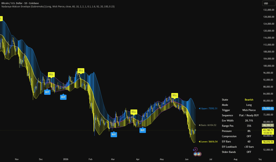
Nadaraya-Watson Envelope [Gabremoku]Nadaraya-Watson Envelope
This indicator builds a non-repainting Nadaraya-Watson envelope using a one-sided Gaussian kernel, so every value is computed from the current bar and past bars only. The goal is to provide a smoother adaptive baseline than a standard moving average while keeping the script operationally honest and suitable for live use.
What makes this script different:
- The central basis is a kernel-weighted Nadaraya-Watson estimate, not a classic SMA/EMA baseline.
- The main envelope is not built from standard deviation by default. It uses kernel-weighted mean absolute deviation (MAD), which is generally less sensitive to single-bar outliers and often produces a more stable channel.
- Standard deviation bands can still be enabled as an optional overlay, so users can compare MAD-based and Stdev-based dispersion around the same kernel basis.
- Signal logic is configurable. Breakout labels can be triggered by close crossing the band, wick piercing the band, or full body breakout, which makes the visual behavior easier to align with the trader’s interpretation.
How it works:
The script applies Gaussian weights to past bars inside the selected window. More recent bars receive the highest weight, while older bars progressively contribute less. The Bandwidth input controls how fast those weights decay. In practice, the effective lookback is usually much shorter than the full Window setting when Bandwidth is low. A practical rule of thumb is that the effective lookback is about 3 × Bandwidth bars, capped by the Window value.
The indicator computes:
1. A kernel-weighted mean, used as the Nadaraya-Watson basis.
2. A kernel-weighted MAD, used as the primary envelope width.
3. An optional kernel-weighted standard deviation, displayed only when the comparison bands are enabled.
The upper and lower MAD bands are then filled with a gradient that increases in strength as price moves away from the basis toward the envelope edges. This makes the visual intensity reflect displacement magnitude, not just bullish or bearish direction.
Compression logic:
The compression zone is based on min-max normalization of envelope width over a lookback period. This is not a statistical percentile rank. A threshold of 0.15 means the current envelope width is near the lower end of the observed width range over the selected compression lookback.
Signal modes:
- Close Cross: triggers only when the close crosses a band.
- Wick Pierce: triggers when the candle’s high or low exceeds a band.
- Body Breakout: triggers when the candle body exceeds a band.
Use Wick Pierce if you want signal labels to match the visible moment where candles extend outside the envelope.
How to use it:
- Use the basis as an adaptive trend reference.
- Use the MAD envelope to judge whether price is stretched relative to recent kernel-weighted behavior.
- Watch compression zones for narrow-range conditions that may precede expansion.
- Compare MAD and Stdev bands when you want to evaluate whether recent volatility is dominated by isolated spikes or by broader dispersion.
Practical notes:
- This script is non-repainting by construction because it does not use centered calculations or future bars.
- Low Bandwidth values create a more reactive basis and shorter effective memory.
- High Bandwidth values create a smoother basis and wider historical influence.
- Increasing Window far beyond roughly 3 × Bandwidth usually has little additional effect.
- Signal labels are state-machine filtered, so they are designed to mark sequence transitions rather than every repeated touch outside the bands.
This indicator is intended as a visual decision-support tool, not as a standalone trading system. It helps traders study adaptive trend, envelope displacement, compression, and breakout structure in a cleaner way than a standard volatility channel. อินดิเคเตอร์
Aegis Kinetic Trend Matrix [wjdtks255]Aegis Kinetic Trend Matrix
■ OVERVIEW
The Aegis Kinetic Trend Matrix is a professional-grade trend-following framework designed to unify macroeconomic bias filters, micro-execution entry triggers, and volatility boundaries into a single, cohesive candle-overlay system.
By integrating three robust open-source concepts—CM_EMA Trend Bars, HalfTrend, and the Nadaraya-Watson Envelope (NWE)—this system provides traders with a multi-layered filtration process to capture structural market swings with precision.
■ KEY FEATURES
CM_EMA Trend Bars: Dynamically shifts candlestick colors based on a 34-period EMA algorithm to isolate core macro direction and eliminate market noise.
HalfTrend Execution Spine: High-precision trailing anchor that tracks micro-trend pivots, offering distinct, instant BUY and SELL execution labels.
Nadaraya-Watson Envelope: Uses non-parametric kernel regression bounds to highlight overextended pricing and filter volatility exhaustion zones at major structural extremes.
■ 개요 (Korean)
Aegis Kinetic Trend Matrix는 거시적 추세 필터링, 미세 타점 포착, 그리고 변동성의 한계 구간을 단 하나의 캔들 오버레이 시스템으로 결합한 하이브리드 트레이딩 프레임워크입니다.
CM_EMA 트렌드 바, 하프트렌드(HalfTrend), 나다라야-왓슨 엔벨로프(NWE) 시스템을 유기적으로 결합하여, 거친 시장 소음을 여과하고 구조적 변곡점을 정밀하게 잡아내도록 설계되었습니다.
■ 핵심 기능
CM_EMA 트렌드 바: 34선 기준 가격 배열에 따라 캔들 색상을 직관적으로 변경하여 시장의 대추세 방향성을 명확히 정의합니다.
하프트렌드 실행 축: 단기적인 마이크로 추세 전환을 정밀하게 추적하며, 즉각적인 BUY/SELL 진입 라벨을 제공합니다.
Nadaraya-Watson 엔벨로프: 커널 회귀 분석 기반의 동적 밴드를 통해 가격의 과도한 이격을 감지하고 추세적 극한 구간의 반전 포인트를 필터링합니다.
■ Credits & Acknowledgments
This indicator is a combined integration based on public domain open-source works. Special credits and gratitude go to the original authors of CM_EMA, HalfTrend, and Nadaraya-Watson Envelope (AlexGrozav) for sharing their invaluable source code with the global community. อินดิเคเตอร์

Volatility Forecast [EXCAVO]Forward Projection of the Bollinger Envelope with Adaptive Horizon and Slope Clamp
The Volatility Forecast takes the classical Bollinger Bands and
projects the basis and the bands forward by a configurable number of bars.
Slopes of the basis, standard deviation and ATR are estimated from linear
regression over a lookback window, then extrapolated through a smooth
curve into the right side of the chart. Small orange dots mark band
reclaim events on confirmed closed bars.
The forecast horizon adapts to the chart timeframe so the projection
stays meaningful at every TF, and a slope clamp prevents the bands from
ballooning into unrealistic territory after sharp regime shifts.
━━━━━━━━━━━━━━━━━━━━━━━━━━━━━━━━━━━━━━━
▸ HOW TO USE
Step 1 → Add the indicator. The current Bollinger Bands are
plotted on the chart and a dashed envelope extends to the
right with the projected basis and bands.
Step 2 → Read the projection. The projected upper and lower
bands show the most likely volatility envelope over the
next bars under the current trend and volatility regime.
Wider end = expansion expected; narrower end = compression.
Step 3 → Use the reclaim dots. A small orange dot below a bar
marks a confirmed bull band reclaim (price tagged the lower
band and pulled back inside). A dot above a bar marks a
bear reclaim. These are context, not entries.
Step 4 → Check the dashboard. The top right panel reads the
projection mode, current width vs its rolling average,
band state, and the last reclaim.
Step 5 → Combine with structure. The envelope pairs well with
trend and structure tools. A breakout that aligns with an
expanding projected envelope tends to continue; one against
a contracting envelope tends to fade.
━━━━━━━━━━━━━━━━━━━━━━━━━━━━━━━━━━━━━━━
▸ HOW IT CALCULATES
◆ Bollinger Bands
Basis is a simple moving average of the source over Length (default 20).
Standard deviation is computed over the same window. Bands are basis plus
or minus Multiplier times standard deviation (default 2.0). These are the
solid plotted lines on the chart.
◆ Linear Regression Slopes
For the projection, the algorithm estimates per-bar slopes from a linear
regression of the basis, the standard deviation, and the ATR over the
Slope Lookback window (default 40). Slope is taken as the difference
between the linreg value at offset 0 and offset 1 - the per-bar drift
the regression expects to continue.
◆ Slope Clamp
Each slope is then clamped to a safety bound so that the cumulative
projected displacement stays sensible. End to end, the projected basis
cannot drift more than two current band-widths, and the projected
standard deviation or ATR cannot grow more than 50% of its current value.
Sign of the slope is preserved so trend direction is intact, only the
magnitude is bounded. This keeps the projection meaningful after sharp
regime shifts.
◆ Forward Projection
Three modes turn slopes into a projected envelope across the forecast
horizon:
Linear extends basis and width on a straight line using the
current slope at every step.
Smooth Curve (default) eases from the current value toward a
dynamic endpoint via a smoothstep curve so the projection has a
natural arc instead of a hard linear extrapolation.
Adaptive Volatility drives the projected width with ATR slope
instead of standard-deviation slope. Useful when volatility is
regime-dependent and the ATR captures it better than stdev.
A projection floor at 50% ensures the envelope never collapses to a
single point on declining-volatility regimes.
◆ Auto Timeframe Forecast
Forecast Bars defaults to Auto, which picks the horizon from the chart
timeframe: 40 bars on 4h and below, 20 on Daily, 10 on Weekly, 6 on
Monthly+. Manual override is available for operators who want a fixed
bar count regardless of timeframe.
◆ Band Reclaim Markers
A bull reclaim fires when the prior bar's low touched the lower band,
the current bar's low has pulled back above the lower band, and the
close sits below the basis. A bear reclaim is symmetric on the upper
band. Cooldown of Length bars prevents same-direction stacking. The
optional Trend MA filter keeps bull marks only above the MA and bear
marks only below. By default markers fire only on confirmed closed bars
(no repaint); Real-time Markers can be enabled if intra-bar feedback is
preferred.
━━━━━━━━━━━━━━━━━━━━━━━━━━━━━━━━━━━━━━━
▸ WHAT MAKES IT DIFFERENT
◆ Adaptive Horizon
The forecast horizon scales with the chart timeframe. The projection
shows a comparable arc on intraday, daily, weekly and monthly without
manual tuning per chart.
◆ Slope Clamp Safety Net
Linear-regression slopes can overshoot after sharp moves or on long
horizons. The clamp caps the cumulative displacement so the projection
cannot grow into unrealistic ranges, regardless of the underlying slope.
◆ Three Projection Modes
Linear, Smooth Curve and Adaptive Volatility cover the common shapes a
volatility envelope can take. Smooth Curve uses smoothstep easing for
a natural arc; Adaptive Volatility ignores stdev drift and tracks ATR
instead.
◆ Confirmed Reclaim Markers
Small orange dots above or below the bar mark band reclaim events. They
fire on confirmed closed bars by default (no repaint), with an optional
real-time mode for operators who prefer intra-bar feedback. A trend-MA
filter keeps the bias clean.
━━━━━━━━━━━━━━━━━━━━━━━━━━━━━━━━━━━━━━━
▸ DASHBOARD
Real-time panel with the current state read:
Mode - Linear / Smooth Curve / Adaptive Volatility
Width vs Avg - current band width relative to its rolling average
Band State - where price sits in the bands (Above Upper / Below Lower / Upper Half / Lower Half)
Last Marker - direction and bars since the last band reclaim
Legend table explains every on-chart element. Both panels toggle in the
Dashboard settings.
━━━━━━━━━━━━━━━━━━━━━━━━━━━━━━━━━━━━━━━
▸ SETTINGS
Bollinger Bands
Source - close (price series used for basis and stdev)
Length - 20 (lookback for basis and stdev)
Multiplier - 2.0 (band width in stdev units)
Basis / Band / Fill Colors - default palette
Forecast Envelope
Forecast Bars Mode - Auto (adapts to chart TF) or Manual
Forecast Bars (Manual) - 40 (used when Mode = Manual)
Slope Lookback - 40 (linreg window for slope estimation)
Mode - Smooth Curve (Linear / Smooth Curve / Adaptive Volatility)
Projection Style / Width / Colors - dashed, default palette
Fill Projection - ON
Reclaim Markers
Show Markers - ON
Real-time Markers - OFF (no repaint by default; closed bars only)
Filter by Trend MA - ON
Trend MA Type - SMA (SMA / EMA / WMA / HMA)
Trend MA Length - 100
Marker Color - orange (#FF8C00)
Show Trend MA - OFF
Dashboard
Show Dashboard - ON
Dashboard Position - Top Right
Show Legend - ON
━━━━━━━━━━━━━━━━━━━━━━━━━━━━━━━━━━━━━━━
▸ ALERTS
Two directional alertconditions are exposed:
Bull Band Reclaim - fires on a confirmed bull reclaim event
Bear Band Reclaim - fires on a confirmed bear reclaim event
Set the alert condition to "Once Per Bar Close" for clean, non-repainting
delivery. Trend-MA filter and cooldown apply to alerts the same way they
apply to the on-chart markers.
━━━━━━━━━━━━━━━━━━━━━━━━━━━━━━━━━━━━━━━
Best regards,
EXCAVO
Disclaimer
Trading involves significant risk. This indicator is a technical analysis
tool and does not constitute financial advice, investment recommendations,
or a guarantee of future results. Past indicator behavior does not
guarantee future performance. Always use proper risk management and your
own judgment.
อินดิเคเตอร์

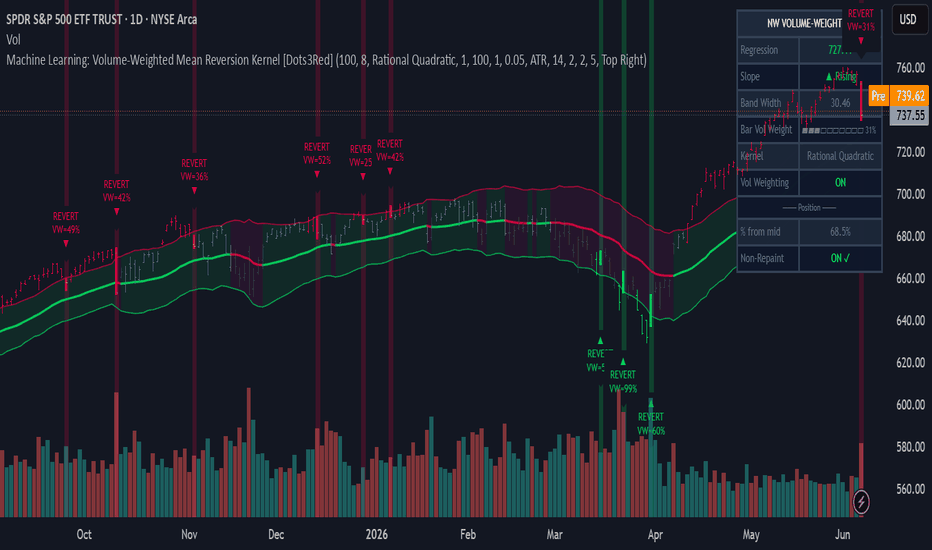
Machine Learning: Volume-Weighted Mean Reversion [Dots3Red]█ MACHINE LEARNING: VOLUME-WEIGHTED MEARN REVERSION KERNEL REGRESSION
Nadaraya-Watson kernel regression is a non-parametric machine learning method. Unlike moving averages which apply fixed, predefined weights to historical bars, kernel regression derives each bar's weight from a mathematical function — the kernel — that measures how relevant that bar is to the current estimate. No hardcoded coefficients. No assumed shape. The model adapts purely from the data.
This script introduces a fundamental extension to the standard method: volume as a second weighting dimension . The result is a regression curve that gravitates toward price levels where real market participation occurred — not toward price levels where a clock happened to tick.
█ WHY KERNEL REGRESSION IS MACHINE LEARNING
The term machine learning describes algorithms that derive structure from data rather than from manually specified rules. Kernel regression satisfies this definition formally. The estimator computes:
ŷ = Σ [ w(i) × close ] / Σ
where each weight w(i) is determined by a kernel function — not by the programmer. The model decides, from the data, how much each historical bar should influence the current estimate. This is the same mathematical family as K-Nearest Neighbors, which weights neighbors by proximity. It is cited as a foundational non-parametric ML method in Bishop (2006) and Hastie et al. (2009), and is described as an attention mechanism in deep learning literature — the same concept behind transformer models. The claim is accurate, not cosmetic.
█ THE CORE INNOVATION — VOLUME WEIGHTING
Every existing Nadaraya-Watson implementation on TradingView uses a pure time kernel:
• Standard NW: w(i) = K(i/h)
This means a bar with 10,000 shares traded and a bar with 10,000,000 shares traded receive identical weight if they are the same number of bars away. A thin overnight drift and a high-volume institutional session influence the regression equally. That is statistically incorrect — volume is a direct measure of how much informational content a price bar carries.
This script uses a volume-weighted kernel:
• This script: w(i) = vol_norm(i) × K(i/h)
where vol_norm(i) is the bar's volume normalized against the peak volume in the lookback window, raised to a configurable power exponent. The regression estimate is therefore:
ŷ = Σ [ vol_norm(i) × K(i/h) × close ] / Σ
High-volume bars anchor the curve. Low-volume bars — thin sessions, overnight drift, holiday trading — contribute minimally. The regression finds where the market actually agreed on price, not just where the clock recorded a tick.
█ THREE KERNEL FUNCTIONS
All three apply the same volume weighting. The choice controls how rapidly influence decays with time distance:
• Rational Quadratic (default) — heavier tail than Gaussian. Bars from 40–60 periods ago still contribute meaningfully if they had high volume. Best for daily and weekly charts where old high-volume levels remain structurally relevant.
• Gaussian — standard bell curve decay. Weight drops sharply with distance. Best for intraday charts where recency matters more than historical anchors.
• Epanechnikov — hard cutoff at the bandwidth boundary. Anything beyond h periods receives zero weight. Produces the most locally sensitive regression. Best for fast charts requiring tight responsiveness.
█ SIGNAL LOGIC
The envelope bands are placed at a configurable multiple of ATR, standard deviation, or a fixed percentage above and below the regression line. Three band width methods are available to match different volatility contexts.
Two signal modes are available:
• Reversion mode (default) — a signal fires when price crosses back through the band after an extension. The ▲ label appears on the bar where price returns inside the lower band. The ▼ label appears on the bar where price returns inside the upper band. This confirms reversion has begun rather than anticipating it.
• Extension mode — enable Signal on extension close to fire a signal the moment price closes outside a band. This is an early warning — useful for alerts before the reversion bar arrives.
Additional signal filters: minimum bars between signals to prevent repeat firing, optional slope direction gate so signals only fire when the regression slope agrees with the signal direction.
█ WHAT YOU SEE ON THE CHART
Regression line
The volume-weighted fair value curve. Cyan when slope is rising, magenta when falling. This is where the model estimates price should be given the recent history of high-participation price levels.
Envelope bands
Upper and lower boundaries built from ATR, standard deviation, or a fixed percentage. The upper band is tinted red — resistance zone. The lower band is tinted green — support zone.
Bar coloring — 4 states
• Bright red — price closed above the upper band. Extended, statistically stretched above fair value.
• Bright green — price closed below the lower band. Extended, statistically stretched below fair value.
• Dim silver — price inside bands, regression rising or falling, i.e normal bullish or bearish context.
The contrast between fully saturated outside-band bars and dimmed inside-band bars makes overextension immediately visible without reading the scale.
Signal labels
▲ REVERT or ▼ REVERT with VW=XX% showing the volume weight of the signal bar. A signal at VW=85% fired on a high-participation bar. A signal at VW=9% fired on a thin bar — lower confidence.
Signal bar highlighting
Two additional layers available: a background flash on the signal bar and a thick vertical line through the bar's full range. Both are independently toggleable. The vertical line uses width=4 — the maximum Pine Script allows — making the signal bar visually distinct even when zoomed out.
Dashboard
Displays: current regression value, slope direction, band width, Bar Vol Weight meter (▰▰▰▱▱▱) showing how much influence the current bar has on the regression, active kernel type, volume weighting status, percentage distance from the regression midline, and non-repainting mode status.
█ NON-REPAINTING
When Non-Repainting Mode is enabled (default), all calculations use a bar offset. The current bar's close does not enter its own regression estimate. Historical signals visible on closed bars will not change as new bars form. Disable this to see a predictive (repainting) version where the current bar participates in its own estimate — useful for visual exploration but not recommended for backtesting or alerts.
█ HOW TO USE
Core use case — mean reversion
This is a mean reversion tool. It works best when price is oscillating rather than trending directionally. The recommended workflow:
1 — Confirm a ranging regime with a separate regime classifier before acting on signals.
2 — Wait for price to reach or pierce the upper or lower band (bars turn bright red or green).
3 — Check the VW% in the signal label. Higher volume weight on the signal bar = higher confidence.
4 — Enter on the reversion signal (▲ or ▼ label). Stop beyond the wick of the signal bar.
5 — Target the regression midline as the primary exit. The % from mid dashboard row tracks progress in real time.
Timeframe guidance
The volume-weighting advantage increases with timeframe because higher timeframes produce more meaningful volume data per bar. H4 and Daily are the strongest timeframes for this tool. For intraday use, reduce the Volume Weight Power to 0.3–0.5 to soften the impact of individual volume spikes.
Quick-start settings by asset class
• Stocks daily: Window=100, Bandwidth=8, Vol Power=1.0, ATR×2.0
• Crypto daily: Window=80, Bandwidth=6, Vol Power=0.7, ATR×1.8
• Forex H4: Window=100, Bandwidth=10, Vol Power=1.0, ATR×1.5
• Indices H1: Window=120, Bandwidth=12, Vol Power=0.8, Stdev×2.0
█ SETTINGS REFERENCE
Kernel Settings
• Lookback Window — number of historical bars in the regression. Larger = smoother, more lag.
• Bandwidth (h) — controls how fast kernel weight decays with time. Higher = older bars still contribute.
• Kernel Type — Gaussian / Rational Quadratic / Epanechnikov. See kernel section above.
• RQ Alpha (α) — Rational Quadratic only. Lower = smoother mixture of length scales.
• Non-Repainting Mode — uses offset. Recommended ON for backtesting.
Volume Weighting
• Enable Volume Weighting — toggle the core innovation on or off. OFF = standard NW.
• Volume Normalization Window — peak volume reference window. Match or exceed the lookback window.
• Volume Weight Power — exponent on the volume weight. 1.0 = linear. 2.0 = quadratic. 0.5 = softer.
• Volume Weight Floor — minimum weight for any bar. Prevents zero-volume bars from being ignored entirely.
Envelope Bands
• Band Width Method — ATR (volatility-adaptive), Stdev (statistical), or Percent (fixed).
• ATR Length — period for ATR calculation.
• ATR / Stdev Mult — multiplier applied to ATR or standard deviation.
• Percent Offset % — used when Percent method is selected.
Signals
• Signal on band crossover — enable signals on band cross events.
• Signal on extension close — fire signal when price closes outside a band (early warning mode).
• Require slope change — only signal when regression slope direction agrees.
• Min bars between signals — gap guard to prevent repeat signals.
Visuals
• Dashboard — regression stats and live metrics table.
• Signal labels — ▲/▼ REVERT labels with volume weight percentage.
• Band fill — fill between upper and lower bands.
• Background flash — bright background color on signal bars.
• Vertical line on signal bar — thick line through full bar height at signal.
• Large dot marker — additional plotchar layer on signal bars.
• Dashboard position — Top Right / Top Left / Bottom Right / Bottom Left.
█ ALERTS
Seven alert conditions are available:
• Long signal — reversion through lower band
• Short signal — reversion through upper band
• Any signal — either direction
• Extended below lower band — early warning before reversion fires
• Extended above upper band — early warning before reversion fires
• Regression slope turned bullish
• Regression slope turned bearish
█ DISCLAIMER
This indicator is a decision-support tool. It does not constitute financial advice and does not guarantee future results. Past statistical patterns do not predict future price behavior. Always use proper risk management.
Method: Nadaraya-Watson Kernel Regression (Non-Parametric ML)
Innovation: Volume × Time Kernel Weighting
Kernels: Gaussian · Rational Quadratic · Epanechnikov
Signals: Mean Reversion (band crossover or extension)
Repainting: Configurable — non-repainting mode available อินดิเคเตอร์
Percentile Stretch Bands [AGPro Series]Percentile Stretch Bands
🔹 OVERVIEW
Percentile Stretch Bands is an empirical, distribution-free overextension map. Instead of plotting standard deviation envelopes that assume a normal distribution of price behavior, this indicator samples the actual historical distance between price and a chosen reference (EMA, VWAP, or Anchored VWAP) and draws context-specific Stretch and Extreme bands directly from the empirical percentile distribution. The result is a visual reference of how stretched price is relative to its own historical behavior, adapted to the asset and timeframe being viewed.
🔹 UNIQUE EDGE
Most "stretch" or "volatility band" tools on the platform rely on parametric assumptions — standard deviation multipliers, ATR multiples, or fixed percentage offsets. These approaches collapse when the underlying return distribution is skewed, fat-tailed, or regime-dependent, which is the rule rather than the exception across crypto and FX assets.
Percentile Stretch Bands takes a different path:
• Distribution-free: bands are drawn from the actual empirical percentile of price-to-reference distance, not from a Gaussian assumption.
• Side-specific sampling: upper and lower distances are collected into separate samples, so asymmetric behavior (trending markets, one-sided regimes) is preserved rather than averaged away.
• Regime-aware rendering: when Focus Active Side is enabled, each bar displays only the side relevant to price position, producing a clean single-story chart without visual competition.
• Readiness gating: bands appear only once a minimum number of observations is reached on the active side, with the status panel clearly indicating the collection stage.
🔹 METHODOLOGY
For every bar in the configured lookback window, the signed percent distance between close and the selected reference is computed and partitioned into two historical samples: positive distances (upper extensions) and negative distances in absolute terms (lower extensions).
Each sample is sorted and two percentile cut-offs are extracted independently:
• Stretch percentile (default 80) — the threshold beyond which a distance is considered materially extended.
• Extreme percentile (default 95) — the threshold beyond which a distance is statistically rare within the chosen lookback.
These cut-offs are then translated from percent-distance back into absolute price bands around the active reference, producing four levels: Upper Stretch, Upper Extreme, Lower Stretch, Lower Extreme. The current distance is also ranked against its side's sample and displayed as an ordinal percentile (for example, "Upper P87") in the status panel.
🔹 SIGNALS AND ALERTS
The indicator is a visual overextension map and does not generate directional trade signals. Four alert conditions are exposed for users who want to be notified of boundary events:
• Upper Stretch Cross — close crosses above the Upper Stretch band.
• Upper Extreme Cross — close crosses above the Upper Extreme band.
• Lower Stretch Cross — close crosses below the Lower Stretch band.
• Lower Extreme Cross — close crosses below the Lower Extreme band.
These alerts mark entries into statistically extended zones relative to the empirical sample. They are contextual flags, not trade recommendations.
🔹 KEY INPUTS
Reference
• Reference Mode — EMA, VWAP, or Anchored VWAP baseline
• EMA Length — smoothing length for the EMA reference
• AVWAP Anchor Time — starting timestamp for Anchored VWAP
Statistics
• Lookback — bars used to build the empirical distribution (default 500)
• Minimum Side Sample — observations required before bands appear
• Stretch Percentile — primary extension threshold (default 80)
• Extreme Percentile — rare-extension threshold (default 95)
Display
• Focus Active Side — regime-aware single-story rendering
• Show Active Stretch Zone Box — right-side zone anchor on the active side
• Zone Forward Projection — forward visibility of the active zone
• Band Color Profile — Soft, Premium, or Bold
• Panel Text Size and Label Text Size — Small, Normal, or Large
Level Tags
• Show Level Tags, Show Reference Tag, Tag Mode, Tag Offset Bars
🔹 HOW TO USE
1. Select a reference that fits the asset and timeframe. EMA is a robust default across all instruments. VWAP is suited to intraday equities and futures. Anchored VWAP is used when a specific event origin (earnings, news, structural low) is relevant.
2. Let the status panel reach the "Ready" state. The panel reports active samples and readiness — bands are intentionally withheld until the side-specific sample is sufficient.
3. Read the current percentile rank in the Zone cell. Values near the center indicate price trading close to the reference; values approaching P95 or above indicate the sample's rare extensions.
4. Treat Stretch and Extreme bands as context, not as triggers. A move into the Extreme zone reflects a statistically rare extension on the chosen sample, not a directional signal.
5. Combine with structural tools — trend context, market structure, higher-timeframe bias — before any discretionary decision.
🔹 LIMITATIONS AND TRANSPARENCY
• The indicator is descriptive, not predictive. Percentile bands describe past behavior within the lookback window; they do not forecast future price action.
• Regime shifts can temporarily invalidate historical bands. A sudden volatility expansion will push price beyond extreme levels while the sample re-stabilizes.
• Empirical percentiles require sufficient observations. On very new symbols or short lookbacks, the "Collecting" state is the correct and expected behavior.
• Anchored VWAP mode depends on a meaningful anchor choice. A poorly chosen anchor produces a reference line without structural relevance.
• The active stretch zone box is a visual anchor for screenshots and review, not a projection of future levels.
🔹 RISK DISCLOSURE
This script is a visual analytics tool and is not a strategy, signal service, or financial advice. It does not place orders, manage positions, or recommend directional exposure. Trading involves risk of loss. Users are responsible for their own analysis, risk management, and trading decisions. อินดิเคเตอร์

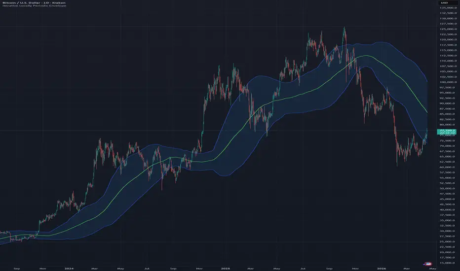
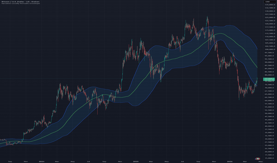
Iterative Locally Periodic EnvelopeThe Iterative Locally Periodic Envelope is a phase-conditioned kernel estimator with temporal locality and endogenous dispersion modeling, implemented as a Nadaraya–Watson estimator under a locally periodic kernel.
The locally periodic kernel defines similarity through cyclical phase alignment modulated by temporal proximity. Observations contribute to the estimator based on both their position within a repeating cycle structure and their recency, emphasizing structural recurrence with sensitivity to local regime conditions.
The indicator computes a latent equilibrium using a kernel-weighted mean and a dispersion measure using kernel-weighted variance under the same weighting structure. The resulting envelope reflects cycle-consistent deviation with temporal locality, rather than a conventional volatility band. All values are computed exclusively on closed historical bars using a bounded lookback window to ensure non-repainting behavior.
This indicator belongs to a broader class of iterative kernel-based envelopes that includes Gaussian, Rational Quadratic, and Periodic variants. All share a common Nadaraya–Watson estimation framework, differentiated by their kernel.
TRADING USES
The Iterative Locally Periodic Envelope is best interpreted as a cycle-aware structural estimator with adaptive temporal sensitivity, rather than a volatility-based band. The temporal locality component allows the estimator to adapt more readily to emerging regime shifts than the pure periodic variant.
Equilibrium Tracking
The latent equilibrium represents the phase-conditioned central tendency of price under locally periodic similarity weighting. Oscillations around this level reflect movement within a repeating structural cycle, with more recent phase-aligned observations contributing more strongly than temporally distant ones.
Cycle Regime Structure
The envelope emphasizes repeating structural behavior through phase recurrence weighting, modulated by temporal decay. Changes in symmetry, amplitude, or persistence of oscillation around the latent equilibrium may indicate transitions between cyclical regimes.
Mean Reversion Within Cycles
When a stable periodic structure is present, deviations from the latent equilibrium may revert toward phase-consistent levels. Mean-reversion behavior is conditioned on both cycle structure and temporal proximity.
Structural Extremes
Extreme deviations relative to the envelope correspond to phase-inconsistent states where cyclical structure becomes stretched or destabilized. Because the kernel incorporates temporal decay, these conditions are identified with greater sensitivity to recent price behavior.
State Estimation
The system defines a latent equilibrium as the inferred central cyclical state under joint phase and temporal weighting, with dispersion derived from kernel-weighted variance under identical constraints. This produces a structurally consistent representation of the market state that is sensitive to both cyclical position and local regime conditions.
LOCALLY PERIODIC ENVELOPE CONSTRUCTION
The envelope is constructed using kernel-weighted variance under the same locally periodic similarity measure used to estimate the latent equilibrium. The latent equilibrium defines the central state estimate and kernel-weighted variance defines dispersion under identical weighting, producing an endogenously determined envelope. The band width is fixed at ±1 kernel standard deviation with no multiplier, ensuring dispersion remains an intrinsic property of the locally periodic similarity structure rather than an externally imposed scaling parameter.
THEORY
The locally periodic kernel defines similarity in terms of cyclical phase recurrence modulated by temporal proximity. Observations contribute to the estimator based on alignment within a repeating cycle structure, with influence attenuated by temporal distance from the estimation point.
The estimator is formulated as a Nadaraya–Watson kernel regression under a locally periodic kernel, where weights are defined as:
k(i) = exp( -2 · sin²(πi / p) / L² ) · exp( -i² / 2L² )
Where:
p = period (cycle length)
L = lookback window (shared bandwidth parameter; effective smoothing scales with L²)
In this MacKay consistent formulation, the lookback window acts as a unified bandwidth parameter governing periodic phase selectivity and the Radial Basis Function (RBF) temporal decay envelope. The two components are coupled through L, producing a kernel that simultaneously emphasizes phase-aligned and temporally proximate observations.
As L increases, both the periodic and RBF components broaden, producing stronger smoothing across phase and time. As L decreases, phase selectivity and temporal locality both increase, making the estimator more sensitive to recent cycle-consistent observations.
This induces a similarity structure in which influence concentrates at phase-aligned intervals within a temporally bounded neighborhood. The resulting estimator defines a latent equilibrium governed by phase alignment and temporal proximity that can be interpreted as a locally stationary periodic extension of kernel regression on a circular phase manifold.
The key distinction from the pure periodic kernel is that phase-aligned observations at distant lags are progressively suppressed by the RBF decay term, allowing the estimator to adapt to structural drift while preserving cycle-aware weighting. During stable cyclical regimes the two estimators converge; during structural transitions the locally periodic variant adapts faster by downweighting older phase information.
CALIBRATION
As established in Gaussian Processes for Machine Learning (Rasmussen & Williams, 2006), the period should reflect the recurrence interval of the dominant cycle in the data, while the bandwidth parameter L controls how quickly similarity decays away from perfect phase alignment. For daily charts, common cycle anchors include the trading week (~5 bars), trading month (~21 bars), trading quarter (~63 bars), and trading year (~252 bars).
Length (Lookback / Bandwidth)
Controls structural depth of the estimator and acts as the unified bandwidth parameter for the periodic and RBF components; as L governs phase selectivity and temporal decay simultaneously, its effect is stronger than in the pure periodic variant. The default of 100 reflects the locally periodic kernel's temporal decay component; at longer lengths the RBF term weakens and behavior converges toward the pure periodic estimator.
- 50–100: high responsiveness, strong temporal locality, short-cycle sensitivity
- 150–250: balanced regime stability with moderate temporal decay
- 300+: broad structural smoothing, weak temporal decay, behavior converges toward pure periodic envelopes
Period (Cycle Length)
Defines the recurrence interval of the kernel and governs phase alignment and cyclical structure. Shorter periods increase phase resolution and cycle sensitivity, while longer periods emphasize broader structural recurrence. The period should reflect the dominant cycle present in the data, aligned with the anchor scales defined above.
Start At Bar
Offsets the kernel window backward from the most recent bars and excludes newer observations from the estimator. This ensures all calculations are based strictly on closed historical data and preserves non-repainting behavior.
MARKET USAGE
Stock, Forex, Crypto, Commodities, and Indices.
Performance is dependent on the presence of stable cyclical structure; in regimes lacking periodic coherence, the estimator converges toward a local smoother with reduced phase discrimination. อินดิเคเตอร์
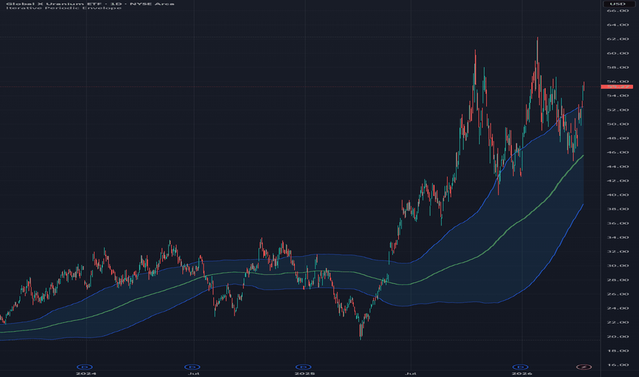
Iterative Periodic EnvelopeThe Iterative Periodic Envelope is a phase-conditioned kernel estimator with endogenous dispersion modeling, implemented as a Nadaraya–Watson estimator under a canonical periodic kernel.
The periodic kernel defines similarity through cyclical phase alignment rather than temporal proximity or multi-scale distance decay. Observations contribute to the estimator based on their position within a repeating cycle structure, emphasizing structural recurrence over linear time dependence.
The indicator computes a latent equilibrium using a kernel-weighted mean and a dispersion measure using kernel-weighted variance under the same weighting structure. The resulting envelope reflects cycle-consistent deviation, rather than a conventional volatility band. All values are computed exclusively on closed historical bars using a bounded lookback window, ensuring non-repainting behavior.
This indicator belongs to a broader class of iterative kernel-based envelopes that includes Gaussian and Rational Quadratic variants. All share a common Nadaraya–Watson estimation framework, differentiated by their kernel.
TRADING USES
The Iterative Periodic Envelope is best interpreted as a cycle-aware structural estimator rather than a volatility-based band.
Equilibrium Tracking
The latent equilibrium represents the phase-conditioned central tendency of price under periodic similarity weighting. Oscillations around this level reflect movement within a repeating structural cycle rather than directional drift.
Cycle Regime Structure
The envelope emphasizes repeating structural behavior through phase recurrence weighting. Changes in symmetry, amplitude, or persistence of oscillation around the latent equilibrium may indicate transitions between cyclical regimes.
Mean Reversion Within Cycles
When a stable periodic structure is present, deviations from the latent equilibrium may revert toward phase-consistent levels. This supports mean-reversion behavior that is conditioned on cycle structure rather than purely statistical dispersion.
Structural Extremes
Extreme deviations relative to the envelope correspond to phase-inconsistent states where cyclical structure becomes stretched or destabilized. These conditions often precede transitions such as cycle inversion, expansion, or compression.
State Estimation
The system defines a latent equilibrium as the inferred central cyclical state, with dispersion derived from kernel-weighted variance under identical periodic similarity constraints. This produces a structurally consistent representation of market state.
PERIODIC ENVELOPE CONSTRUCTION
The envelope is constructed using kernel-weighted variance under the same periodic similarity measure used to estimate the latent equilibrium. The latent equilibrium defines the central state estimate and kernel-weighted variance defines dispersion under identical weighting, producing an endogenously determined envelope. The band width is fixed at ±1 kernel standard deviation with no multiplier, ensuring dispersion remains an intrinsic property of the periodic similarity structure rather than an externally imposed scaling parameter.
THEORY
The periodic kernel defines similarity in terms of cyclical phase recurrence rather than linear temporal distance. Observations contribute to the estimator based on alignment within a repeating cycle structure.
The estimator is formulated as a Nadaraya–Watson kernel regression under a canonical periodic kernel, where weights are defined as:
k(i) = exp( -2 · sin²(πi / p) / L² )
Where:
p = period (cycle length)
L = lookback window (bandwidth parameter; effective smoothing scales with L²)
In this MacKay consistent formulation, the lookback window acts as a bandwidth control parameter, governing phase selectivity and structural smoothing. As L increases, the kernel becomes broader, producing stronger smoothing and reduced phase sensitivity. As L decreases, phase selectivity increases and the estimator becomes more locally sensitive to cyclical alignment.
This induces a cyclical similarity structure in which influence concentrates at recurring phase intervals. The resulting estimator defines a latent equilibrium governed by phase alignment rather than temporal proximity. This formulation can be interpreted as a periodic extension of kernel regression on a circular phase manifold.
CALIBRATION
Length (Lookback / Bandwidth)
Controls structural depth of the estimator and acts as the primary kernel bandwidth parameter.
- 50–100: high responsiveness, short-cycle sensitivity
- 150–250: balanced regime stability
- 300+: strong structural smoothing, reduced sensitivity to phase noise
Period (Cycle Length)
Defines the recurrence interval of the kernel and governs phase alignment and cyclical structure. Commonly aligns with dominant market rhythms such as intraday or macro-cycle structure.
- Lower values: faster cycle sensitivity
- Higher values: slower, broader structural cycles
Start At Bar
Offsets the kernel window backward from the most recent bars and excludes newer observations from the estimator. This ensures all calculations are based strictly on closed historical data and preserves non-repainting behavior.
MARKET USAGE
Stock, Forex, Crypto, Commodities, and Indices.
Performance is dependent on the presence of stable cyclical structure; in regimes lacking periodic coherence, the estimator converges toward a smoother, low-information state. อินดิเคเตอร์
AG Pro ATR Envelope Breakout Quality [AGPro Series]AG Pro ATR Envelope Breakout Quality
Overview / What it does
AG Pro ATR Envelope Breakout Quality is a volatility-aware breakout framework built around a dynamic ATR envelope rather than a static horizontal level, fixed box, or session-defined range. The script tracks when price closes outside an ATR-based outer band, then evaluates whether that move shows enough quality to be treated as a meaningful breakout instead of a weak expansion, short-lived overshoot, or low-conviction push.
The core logic is centered on three linked questions. First, did price achieve a valid close outside the active envelope? Second, was that move supported by enough momentum and relative participation to deserve attention? Third, what happened when price came back toward the broken area? This progression allows the script to move beyond a simple breakout marker and present a more structured breakout-quality workflow.
Because the reference structure is dynamic, the script adapts to changing market conditions instead of forcing all setups into a fixed box logic. In periods of contraction, the envelope tightens and makes outside acceptance more meaningful. In periods of expansion, the envelope widens and helps separate true continuation pressure from ordinary volatility noise. This makes the tool especially useful for traders who want to judge whether an expansion is merely visible or genuinely tradable.
The visual design is intentionally clean and overlay-first. The envelope defines the active volatility shell, breakout markers show where price escapes that shell, the throwback zone highlights the key acceptance pocket after the move, and the optional target line provides a simple expansion objective. A compact panel then summarizes the current state without taking over the chart. The result is a script that aims to look premium while still keeping the main story readable in a publish screenshot.
Unique Edge
The main distinction of this script is that it does not evaluate breakout quality from a static support/resistance line, a consolidation rectangle, a Donchian extreme, or an opening range boundary. It evaluates breakout quality from a moving ATR envelope. That difference is not cosmetic. It changes the entire logic of what counts as a breakout, how follow-through is judged, and how retests are interpreted.
In several classic breakout tools, the market is asked to escape a fixed historical structure. Here, the market is asked to achieve acceptance outside a live volatility shell. This creates a different analytical lens. A move that looks impressive relative to a flat level may not be meaningful relative to a volatility-adjusted envelope. On the other hand, a clean close outside an adaptive outer band can reveal expansion quality that a simple line break would miss.
This also separates the script from our other AG Pro tools. It is not a consolidation breakout evaluator, because its reference structure is not a box. It is not a Donchian breakout tool, because it is not based on period highs and lows. It is not an opening-range breakout model, because it is not session-box dependent. It is not a standard break-retest script, because the retest here happens around a dynamic envelope acceptance area rather than around a static horizontal level.
That distinction matters both analytically and visually. Analytically, the script focuses on volatility-adjusted breakout acceptance. Visually, it produces a different type of chart story: an active envelope, a breakout event, a throwback pocket, and a projected path. This gives the script its own place inside the AG Pro catalog rather than making it feel like a variation of an existing breakout family member.
Methodology
The script begins with an ATR-based envelope built around a moving basis. This creates an adaptive upper and lower band that expand or contract with market volatility. A bullish breakout candidate appears when price closes outside the upper band. A bearish breakout candidate appears when price closes outside the lower band. Wick-only excursions are not enough. The script is designed to care about acceptance, not mere contact.
Once an outside close is detected, the script evaluates breakout quality through a compact scoring framework. Momentum contribution helps measure whether the breakout candle shows real displacement or just a hesitant push. Volume contribution helps detect whether the breakout is supported by stronger-than-usual participation or whether it lacks confirmation. The combined result becomes the displayed breakout-quality score.
After the initial breakout, the script monitors the first return toward the broken band area. This is where the throwback logic becomes important. Instead of treating every pullback the same way, the script classifies what happens around the envelope area and updates the state accordingly. A successful hold suggests that the market accepted the breakout. A failure suggests that the move lost structural quality after the initial expansion.
An optional target line can be used to project a simple post-breakout objective. This is not presented as a promise of outcome. It is a visual planning reference intended to show a possible expansion path if the breakout continues to behave constructively. Together, the envelope, the breakout signal, the throwback state, and the target framework create a full breakout-quality sequence rather than a single event label.
Signals & Alerts
The script is designed to organize the breakout workflow into visible states rather than flooding the chart with constant commentary. The main states include bullish breakout, bearish breakout, throwback monitoring, throwback hold, breakout failure, and target hit. This makes the chart easier to read and helps the user understand where the setup currently stands.
Bullish and bearish breakout markers appear when price achieves a confirmed outside close beyond the relevant envelope band. These are the initial expansion events. They are then followed by a monitoring phase in which the script watches how price behaves around the broken band area. If the return is constructive, the script can label that behavior as a successful hold. If the move loses quality and breaks down, the script can classify it as a failure.
The target marker is optional and functions as a planning aid, not as a certainty engine. It simply shows that the projected expansion objective has been reached based on the chosen configuration. In practical use, this can help traders separate the breakout event itself from the later progression of the move.
The alert set is intended to remain deterministic and chart-state aware. It focuses on confirmed breakout events, throwback behavior, breakout failure, and target completion. This keeps the script aligned with workflow clarity instead of turning it into a noisy alert generator.
Key Inputs
The envelope settings control the moving basis, ATR length, and multiplier that define the adaptive breakout shell. These settings determine how sensitive the script is to changing volatility and how demanding the outside-close condition becomes.
The breakout filter settings allow the user to regulate confirmation quality. Depending on the selected configuration, the script can require stronger momentum, clearer outside distance, and optional volume confirmation. This helps users decide whether they want a more selective or more responsive model.
The throwback analysis settings define how the script interprets the first return toward the broken envelope area. These settings influence how deeply price can revisit the area before the move is treated as weak, failed, or still acceptable.
The target settings control whether the projected objective is shown and how far it is placed from the breakout area. The visual settings then manage panel visibility, panel placement, font sizing, historical object behavior, and label density so the script can remain clean in live use and in publish screenshots.
Limitations & Transparency
This script is a breakout-quality framework, not a prediction engine. It does not know in advance whether a breakout will continue. It evaluates the quality of a breakout after a valid outside-close event occurs and then tracks how price behaves afterward. That distinction is important.
The ATR envelope is an adaptive reference, which means the same market move may be classified differently under different volatility regimes. That is intentional. The script is designed to respond to changing market structure, but any adaptive model will also reflect the sensitivity of its settings. Users should therefore expect the behavior of the tool to vary across symbols, timeframes, and volatility environments.
Volume inputs may also behave differently across markets and data feeds. On some instruments, volume can add useful confirmation. On others, it may be less informative. For that reason, volume should be treated as a supporting factor rather than as an absolute truth layer.
The target projection is a chart-planning feature, not a guaranteed outcome. Likewise, a breakout failure label does not mean the market cannot later recover, and a target hit does not mean the move was universally optimal. The script is meant to help structure chart reading, not replace trade management, context analysis, or personal decision-making.
How this script differs from our other AG Pro tools
Within the AG Pro lineup, this script is intentionally positioned as a volatility-envelope breakout tool. It does not compete with our box-based breakout logic, our period-high/low breakout logic, or our static break-retest logic. Its role is to answer a different question: did price achieve meaningful acceptance outside an adaptive ATR shell, and did that acceptance survive the first return test?
That makes it especially useful when traders want a volatility-adjusted view of expansion quality. In markets where static levels are repeatedly pierced, an adaptive envelope framework can provide a cleaner read on whether the move is truly escaping current volatility conditions or simply stretching within ordinary noise.
In that sense, the script is not a replacement for our other breakout-oriented tools. It is a separate layer with a different reference model, different retest logic, and a different chart story. That separation is deliberate and is one of the reasons the script belongs in its own category inside the broader AG Pro collection.
Risk Disclosure
This script is an analytical chart tool designed to visualize volatility-adjusted breakout conditions, breakout quality, and post-breakout behavior. It is not financial advice, not a signal service, and not a guarantee of future price direction.
All breakout conditions can fail. Momentum can fade, volume can be inconsistent, and throwback behavior can change quickly. Markets remain uncertain, and no indicator can eliminate risk. Users should always apply their own market judgment, risk controls, and execution rules.
Use the script as a structured decision-support layer, not as a stand-alone trading instruction. Confirmation from broader context, trend conditions, liquidity structure, and personal risk management remains essential.
อินดิเคเตอร์

CAP Channel Trading (Auto-Deviation & Analysis Dashboard)This indicator is a highly precise and comprehensive replica of the well-known "MeetAlgo CAP Channel Trading" indicator, originally developed for MetaTrader 4 and 5. It has been built from the ground up in Pine Script v6 and expanded with exclusive TradingView features (such as Auto-Deviation calculation and dynamic themes).
The indicator is based on the "Advanced Envelope Theory." This theory assumes that market prices naturally oscillate within dynamically calculated boundaries (envelopes). If the price breaks out of these boundaries or touches them, it signals a statistical anomaly and provides an excellent opportunity for reversal trades.
Unlike classic Bollinger Bands, which often lag behind volatility, this system reacts extremely sensitively to current fluctuations and keeps the channel width much more constant.
🧠 How does the indicator work?
The Center Line (TMA): The heart of the channel is a double-smoothed Triangular Moving Average. This filters out short-term market noise and forms a static center of gravity for the price.
The Outer Bands (ATR): The channel boundaries are calculated using the Average True Range (ATR) as a proxy for true market volatility.
Auto-Deviation (Exclusive): Since highly volatile instruments (like XAUUSD on the 5M chart) have more extreme outliers than quiet Forex pairs, this indicator features an Auto-Deviation logic. It analyzes the last 200 candles and calculates the 85th percentile of volatility to stretch the channel exactly enough to capture normal price action, while immediately providing razor-sharp signals during real breakouts.
✨ Main Features & Visualization (See Screenshots)
Dual-Color Smart Bands: The channel visually displays the market state. If the price remains safely within the channel, the bands are red with a yellow edge. If the price touches the outer boundary and enters the reversal zone (Overbought/Oversold), the bands instantly switch to black with a green edge.
Precise Entry Signals: As soon as extreme zones are reached, the indicator plots colored arrows (including the exact entry price as text) directly above or below the corresponding candle. The text color automatically adapts to your TradingView theme (Light/Dark).
Live Analysis Dashboard: In the top right corner of the chart, there is an info table that automatically simulates trades in the background and evaluates how profitable the signals currently are (including Win-Rate, accumulated Points/Pips, and the Live Spread).
⚙️ Settings (Parameters)
1. Auto-Calculate Optimal Deviation
(Default: Enabled) Allows the indicator to independently calculate the optimal channel width (Deviations) for the currently open instrument and selected timeframe. Ideal for dynamic markets like Gold.
2. Auto-Dev Percentile (Sensitivity)
(Default: 85) Controls the sensitivity of the automatic calculation. A lower value (e.g., 80) ignores more historical spikes, makes the channel tighter, and generates signals more frequently. A higher value (e.g., 95) makes the channel wider and filters signals more strictly.
3. Auto-Dev Smoothing Length
(Default: 14) Smooths the dynamically calculated channel width using an Exponential Moving Average (EMA). This prevents the channel from becoming erratic during a sudden, unnatural price spike.
4. Static Deviations
(Default: 2.0) The manual multiplier for the distance of the bands to the center line. This value is only used if the "Auto-Calculate" function is disabled.
5. Trade Exit Level
Determines at which point the dashboard considers a trade "closed" to calculate the Win-Rate.
Middle Line (Default): A trade is opened at the outer band and closed exactly at the TMA center line.
Opposite Band: A trade is only closed when the price has traveled completely through the channel and touches the opposite band.
6. Show Analysis Report
Shows or hides the performance dashboard (Info-Box) in the top right corner of the chart.
7. Signal Bar (Notification)
ClosedBar (Default): Signals and dashboard evaluations are only confirmed when the current candle has completely closed. This prevents "repainting" (arrows disappearing later).
LiveBar: Evaluates every tick in real-time. Can enable faster entries but carries the risk of false signals if the price pulls back before the candle closes. อินดิเคเตอร์

LOWESS Adaptive Envelope [BackQuant]LOWESS Adaptive Envelope
Overview
LOWESS Adaptive Envelope is a nonparametric trend-fit and volatility envelope tool built around LOWESS (Locally Weighted Scatterplot Smoothing). Instead of smoothing price with a fixed-form moving average, this indicator performs a rolling set of local weighted linear regressions across a chosen historical window and stitches those local fits into a single smooth curve that adapts to changing market structure.
On top of the fitted curve, the script builds an adaptive envelope whose width is driven by the local magnitude of the model’s residuals (how far price deviates from the fit). That means the envelope automatically expands when the market is noisy or trending aggressively, and contracts when price is stable or mean-reverting cleanly.
The output is a complete “structure map”:
A LOWESS fitted centerline (trend estimate).
Upper and lower adaptive bands derived from smoothed residual spread.
A filled region that changes color based on where price sits relative to the fit.
Optional extrapolation of the fit and envelope into the future using last slope, with widening uncertainty.
An info label showing fit quality (R²), position inside the envelope, and direction.
Where LOWESS comes from (and why it is different from moving averages)
LOWESS (also written LOESS) is a classic statistical smoothing technique used in exploratory data analysis and robust curve fitting. It became popular because it can approximate complex shapes without assuming a single global model. Instead of forcing the entire window to follow one equation (like a single linear regression or a single moving average kernel), LOWESS fits many small local regressions , each one tailored to its neighborhood.
Key distinction:
A moving average is a fixed smoother, it applies the same weighting rule everywhere, regardless of whether the market is trending, chopping, or accelerating.
LOWESS is a locally re-fitted model, it re-estimates slope and intercept at each point based on nearby data.
In price terms:
LOWESS is better at “hugging structure” when the market curves or transitions.
It can follow gradual regime shifts without the same lag profile as long-window MAs.
It does not assume the trend is constant across the whole lookback, it assumes trend can vary locally.
What the indicator is modeling
Think of the lookback window as a dataset of points:
x = bar index (0..length-1 inside the window)
y = price
For every point i inside that window, the indicator estimates the best local line:
y ≈ a + b * x
But it does this using only nearby points, and it weights them by distance from i. So the fitted value at i is a locally weighted regression prediction.
The final fitted curve is the collection of those predictions across i = 0..length-1.
Core mechanics: local weighted linear regression
1) Neighborhood size (bandwidth)
The “locality” is controlled by a bandwidth parameter. In this script:
h = max(bandwidth * length / 2, 2)
Interpretation:
h acts like a radius measured in bars inside the fitting window.
Lower bandwidth → smaller h → more local fit (more responsive, can track curvature, more sensitive to noise).
Higher bandwidth → larger h → more global fit (smoother, more stable, more lag in transitions).
So bandwidth controls the bias-variance tradeoff:
Small bandwidth: low bias, high variance.
Large bandwidth: higher bias, lower variance.
2) Tricube kernel weighting
LOWESS requires a weight function that decays smoothly with distance. This script uses the classic tricube kernel :
For each candidate point j around target i:
u = |i - j| / h
If u < 1:
- w = (1 - u³)³
If u ≥ 1:
- w = 0
Why tricube:
Weights go to zero smoothly at the boundary (no sharp cutoff artifacts).
Nearby points dominate the fit, distant points contribute little or nothing.
It is a standard LOWESS choice because it produces stable smooth curves.
3) Weighted least squares fit
For each i, the script accumulates weighted sums over j in the neighborhood:
sumW, sumWX, sumWY, sumWXX, sumWXY
These correspond to the normal equations for weighted linear regression. From those, it computes:
denom = sumW * sumWXX - sumWX²
a and b derived from sums (intercept and slope)
fitted = a + b * i
If denom is too small (numerical instability, insufficient variation), it falls back to the raw price at that i.
This entire process is repeated for every i in the window, which is why it is done only on the last bar (performance).
Why it fits inside the window rather than a single line
A single regression across 200 bars assumes one slope b explains the whole move. Markets rarely do that. LOWESS allows the slope to drift through time, which is exactly what “trend structure” actually does in real price.
Residuals: turning model error into volatility structure
Once the LOWESS fitted curve is computed, the script measures the residual at each point:
res = price - fitted
Residuals are the model’s error. In trading terms, residual magnitude is a proxy for:
Local noise level.
Deviations from trend structure (overextension/underextension).
Regime instability (trend is less “explanatory”).
The script takes absolute residuals:
absRes = |res |
This is important because envelope width should reflect spread size regardless of direction.
R²: fit quality and regime information
The indicator also computes R² over the window:
ssRes = Σ(res²)
ssTot = Σ((price - meanPrice)²)
R² = 1 - ssRes/ssTot
Interpretation:
Higher R² means the LOWESS fit explains more of the variation inside the window.
Lower R² means price is behaving in a way the smooth trend model cannot explain well (chop, shocks, irregular volatility).
In markets, R² can be read as “how trend-like vs how noisy” the recent environment is, but remember it depends on your chosen length and bandwidth.
Adaptive envelope construction (what makes it “adaptive”)
A normal envelope uses a constant width (like ±k*ATR or ±k*stdev). This script does something different: it estimates a local envelope width based on smoothed residual magnitude.
1) Smooth residual magnitude locally
It computes a residual averaging window:
rWin = max(3, int(h * 0.8))
So the residual smoothing window is linked to the LOWESS locality. If the fit is local, the envelope adapts locally. If the fit is global, the envelope adapts more slowly.
Then for each i:
envW = mean(absRes over ) * envMult
Interpretation:
The envelope width is proportional to how much price typically deviates from the fit around that region.
envMult is your “how many spreads” multiplier.
This creates an envelope that expands and contracts along the curve, not a single constant band.
2) Upper and lower envelopes
For each i:
upper = fitted + envW
lower = fitted - envW
This is a model-driven channel. It is not ATR-based directly, it is “error-based.” That makes it very effective at responding to the actual behavior of the market relative to the fitted structure.
How to interpret the envelope
The centerline is the best local structural estimate. The envelope is the expected deviation range around that structure.
Typical readings:
Price near centerline: balanced relative to structure.
Price riding upper band: strong bullish pressure, trend continuation or overextension depending on context.
Price riding lower band: strong bearish pressure, continuation or overextension.
Repeated band rejections: mean-reversion regime around the structural fit.
Envelope widening: instability rising, volatility expanding, structure less reliable.
Envelope tightening: compression, cleaner trend or coiling behavior.
Because the band width is based on residuals, widening often coincides with “trend breaks” and regime transitions, not just higher ATR.
Color logic and visual encoding
The envelope fill color is based on price relative to the most recent fitted value:
If close > fitted , bullish color.
Else bearish color.
So color is a regime/bias cue, not a volatility cue. The bands themselves are drawn with translucent versions of the same regime color, while the fit line is a subtle white.
The fill polygon is constructed by:
Walking forward through upper points.
Then walking backward through lower points.
So the shape is closed and can be filled cleanly using polyline fills.
Extrapolation: forward projection with widening uncertainty
This script can project the fitted line into future bars. This is not forecasting in a statistical sense, it is a deterministic extension based on the current slope.
How it extrapolates
It takes:
slope = fitted - fitted
lastFit = fitted
Then for i = 1..extrapBars:
futureFit = lastFit + slope * i
This is a linear continuation of the most recent fit direction. It is meant as a visual guide for “if the current local trend continues.”
Why the forward envelope widens
The script also grows the envelope slightly with each projected bar:
envGrow = lastEnv * 0.01
futureEnv = lastEnv + envGrow * i
This is a simple uncertainty widening mechanism. As you move further into the future, you should assume less confidence. The envelope expansion encodes that visually without claiming statistical rigor.
Info label: what it reports and how to read it
When enabled, the label shows:
1) Direction arrow
It computes a slope over the last few fitted points:
recentSlope = fitted - fitted (or closest valid index)
▲ if slope >= 0
▼ if slope < 0
This gives a slightly more stable direction read than one-bar slope.
2) R²
Displayed as R²: 0.xxx, representing how well the LOWESS curve explains window variation.
3) Envelope Position (Env Pos)
It measures where the current close sits inside the latest envelope:
0% = at lower band
50% = at centerline
100% = at upper band
This is extremely useful as a normalized “over/under extension” metric because it is scaled by the adaptive band width, not raw price units.
How to use it properly
Trend structure and regime filtering
Use the fit line as structural trend direction.
Use the fill color as quick bias context.
Use R² as a “trend quality” read: high R² tends to mean cleaner structure, low R² tends to mean chop or instability.
Mean reversion vs continuation
This tool can support both styles, but interpretation differs:
Mean reversion framing
If market repeatedly returns to the fit line, the fit is acting like value.
Upper band touches can be “overbought relative to structure.”
Lower band touches can be “oversold relative to structure.”
Envelope position becomes your normalized stretch gauge.
Trend continuation framing
In strong trends, price can ride a band rather than revert to centerline.
Band riding plus rising fit slope suggests persistence.
A sudden failure to hold the band plus falling R² can flag transition risk.
Breakdown/transition identification
Because the envelope width is residual-driven:
If price starts producing large residuals, the envelope expands.
That expansion is often a signature of regime change, not just volatility.
Combine expansion with slope flattening to identify trend exhaustion.
Parameter tuning (what each input really does)
Length
Defines how much historical data is used for the full fit. Larger length:
More stable curve.
More computational load.
Tends to represent macro structure.
Bandwidth
Controls locality:
Low bandwidth (0.10–0.25): more reactive, tracks curvature and micro-structure, more sensitive to noise.
Higher bandwidth (0.30–0.50+): smoother, more stable, more lag in fast turns.
Envelope Width (envMult)
Scales how wide the adaptive band is relative to the local residual spread:
Lower values create a tighter channel, more band interactions.
Higher values create a wider channel, fewer touches, better for regime filtering.
Extrapolation Bars
Purely visual. More bars gives a longer projected structure line and uncertainty region.
Limitations and correct expectations
LOWESS is powerful, but it is not a magic predictor.
LOWESS is descriptive, it fits what happened, then projects linearly if extrapolation is enabled.
In sudden shocks or gaps, the fit will update only after the new data is inside the window.
Very small bandwidth can overfit local noise, producing misleading curvature.
Very large bandwidth can underfit, behaving like a slow regression and missing turning points.
R² is window-dependent, a low value does not mean “bad indicator,” it often means “market is not smooth right now.”
Summary
LOWESS Adaptive Envelope applies locally weighted linear regression (LOWESS) with a tricube kernel to build a smooth, structure-following fitted price curve that adapts to regime changes without relying on a fixed moving-average form. It then converts the model’s local residual spread into a dynamic envelope that expands and contracts with real deviation behavior, provides fit quality via R², normalizes price position inside the band, and optionally extrapolates the latest structural slope forward with widening uncertainty. The result is a robust trend-structure and deviation framework that is equally useful for regime filtering, mean-reversion context, and trend persistence assessment. อินดิเคเตอร์
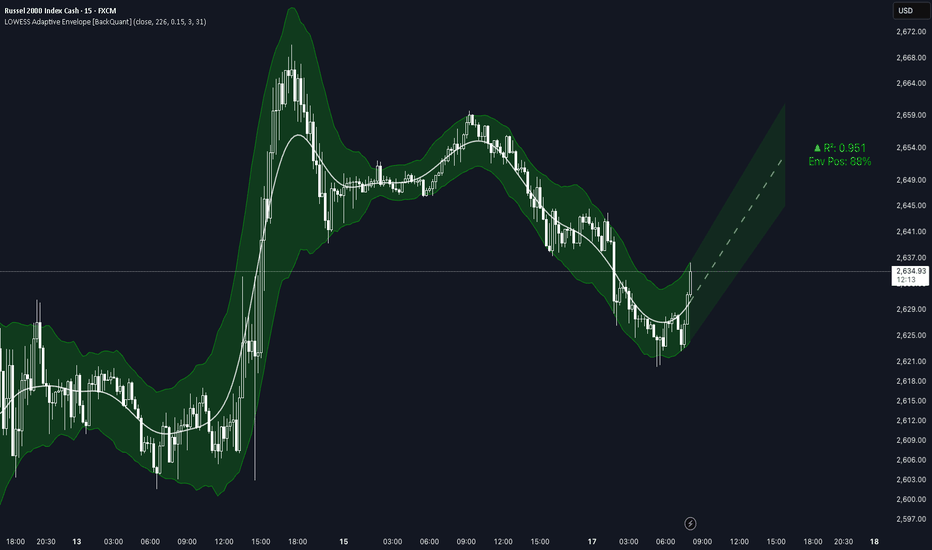
Whittaker Envelope [LuxAlgo]The Whittaker Envelope indicator is a visualization tool that uses Asymmetric Least Squares (ALS) to create a smooth, non-linear envelope that adapts to price extremes and troughs.
This indicator is for visualization purposes only and should not be used for direct trading signals without confirmation.
It is important to note that this script is displayed retrospectively . Because it calculates the best fit over a fixed historical window (the last N bars) using an iterative optimization process, the entire shape of the envelope can change as new data arrives. This means the indicator repaints and should be used to analyze overall market structure and volatility rather than for real-time execution.
🔶 USAGE
The Whittaker Envelope provides a unique way to visualize the "breathing" of the market. By applying different asymmetry parameters, the indicator generates a lower boundary that seeks out price troughs and an upper boundary that seeks out price peaks.
🔹 Trend and Volatility Analysis
The area between the upper and lower bounds represents the smoothed price range. A widening envelope suggests increasing volatility, while a narrowing one indicates consolidation. The dashed midline acts as a smoothed average of these two extremes, providing a baseline for the current trend.
🔹 Extrapolation
The tool includes a linear extrapolation feature that projects the current trajectory of the envelope into the future. This can help users visualize the potential direction of the trend if the current momentum persists.
🔶 DETAILS
The script implements the Whittaker-Eilers smoothing algorithm, which balances two conflicting goals: fitting the data points closely and keeping the resulting curve smooth.
By using Asymmetric Least Squares (ALS), we assign different weights to prices depending on whether they are above or below the curve. For the upper band, we use a high asymmetry value ( p ) so the curve is "pushed" toward the peaks. For the lower band, a very low p value is used to "pull" the curve toward the troughs.
🔶 SETTINGS
Length : The number of recent bars included in the calculation window.
Lambda (λ) : The smoothing factor. Higher values result in a stiffer, straighter envelope, while lower values allow the bands to follow price more closely.
Lower Asymmetry (p) : Controls how the lower band reacts to prices. Typically set to a very low value (e.g., 0.001) to ensure it follows the bottom of the price action.
Upper Asymmetry (p) : Controls how the upper band reacts to prices. Typically set to a very high value (e.g., 0.999) to ensure it follows the top of the price action.
Iterations : The number of times the ALS algorithm runs to refine the fit. More iterations provide a more accurate envelope but require more computational power.
Extrapolation : The number of bars to project the current slope of the bands into the future.
Source : The price data used for the calculation (default is Close).
อินดิเคเตอร์

Adaptive Nadaraya-Watson (Non Repainting) [Metrify]To understand this implementation of the Nadaraya-Watson estimator, we have to look at the core equation governing non-parametric regression. This script aren't trying to average prices; we are trying to find the probability density of where price should be relative to its recent history.
1. The Kernel Physics (Bandwidth Modulation)
In standard kernel regression, you have a bandwidth parameter (h). This controls the "smoothness" of the curve. If h is too low, the curve jitters with every tick of noise. If h is too high, it acts like a sluggish SMA.
A static h fails because market volatility is dynamic. When the market explodes (high volatility), a tight bandwidth generates false signals. When the market sleeps, a wide bandwidth misses the micro-trends.
It try solving this by making h a function of the Asset's volatility ratio:
heff=h×max(0.5,min(SMA(ATR20,100)ATR20,2.0))
If the current ATR(20) is double the long-term average (100), the bandwidth doubles. This forces the estimator to "zoom out" during chaos, effectively ignoring noise that would otherwise look like a reversal.
vol_ratio = use_vol ? vol_raw / (vol_base == 0 ? 1 : vol_base) : 1.0
vol_mod = math.max(0.5, math.min(vol_ratio, 2.0))
h_eff = h_val * vol_mod
2. The Gaussian Loop (Endpoint Estimation)
Standard Nadaraya-Watson scripts repaint because they calculate the regression over a full window centered on the bar. To make this usable for live trading, we must calculate the Endpoint Estimate.
We iterate backward from the current bar (i=0) to the lookback limit. For every historical price Xi, we calculate a weight wi based on how far away it is in time (distance).
The weight is derived from the Gaussian Kernel function:
wi=exp(−2heff2i2)
Price data closer to the current bar (i=0) gets a weight near 1.0. Data further away (i=50) decays exponentially toward 0.
for i = 0 to lookback by 1
float dist = float(i)
float w = math.exp(-math.pow(dist, 2) / (2 * math.pow(h_eff, 2)))
num := num + w * src
den := den + w
3. Statistical Deviation (MAE vs. StDev)
Most Bollinger Band-style indicators use Standard Deviation (Root Mean Square). The problem with StDev is that it squares the errors, which heavily penalizes large outliers. In crypto or volatile forex pairs, one wick can blow out the bands for 20 bars.
This one use Mean Absolute Error (MAE) instead.
MAE=N1∑∣Price−y^∣
MAE is linear. It measures the average distance price strays from the kernel estimate without squaring the penalty. This creates "tighter" bands that adhere closer to price action during normal trend behavior but don't expand ridiculously during a flash crash.
Pine Script
float error = math.abs(src - y_hat)
float mae = ta.sma(error, lookback)
We project two sets of bands:
Inner Band (Balanced): The "Noise Zone". Price inside here is considered random walk.
Outer Band (Precision): The "Exhaustion Zone". Price reaching here is statistically unlikely (2.8x MAE).
Input & Visual Summary
Kernel Physics:
h_val: The base smoothness. Lower (e.g., 6) = faster, noisier. Higher (e.g., 10) = slower, smoother.
use_vol: Keep this TRUE. It prevents the bands from being too tight during news events.
Envelope Statistics:
mult_in / mult_out: These are your risk settings. 1.5/2.8 is a standard deviation-like setting suited for MAE.
อินดิเคเตอร์

VDUB Bands - MTF WMA+ATR Volatility Lanes (6 Alerts)VDUB Bands draws volatility-scaled “trend lanes” around a Weighted Moving Average (WMA) using ATR (or a WMA of True Range). It can display up to four tiers (L1–L4), with higher tiers sourced from higher timeframes to show local structure → higher-timeframe structure on a single chart.
────────────────────────────────────────
1. What it does (plain English)
────────────────────────────────────────
Think of each tier as a lane system around the trend:
• Inner rails = “normal volatility lane” around the WMA
• Outer rails = “extension / extreme zone” for that tier
• Higher tiers (L3/L4) show bigger structure
• Lower tiers (L1/L2) show active lane behavior
Typical interpretation:
• Price inside inner rails → normal variance around the trend lane
• Between inner and outer → stretched, but not extreme
• Outside outer rails → extended vs that tier’s volatility band
────────────────────────────────────────
2) Why it’s useful (and why it’s not a mashup)
────────────────────────────────────────
This is not a bundle of unrelated indicators. Everything serves one cohesive purpose:
• Visualize trend + volatility lanes across multiple time horizons
• Keep rails consistent and readable (levels, fills, outlines)
• Optional multi-timeframe aggregation for structure context
• A compact 6-alert set to catch key transitions without alert spam
────────────────────────────────────────
3) What you see on the chart
────────────────────────────────────────
For each level (L1–L4), you can show:
• Upper/Lower Inner rails
• Upper/Lower Outer rails
• Optional center fill (between outer rails) = operating range
• Optional MA line per tier (off by default to reduce clutter)
• Base WMA line (L1 MA) if enabled
Suggested workflow:
• Start with L1 + L2 only
• Add L3/L4 once you like the structure view
• Use Dynamic Opacity if the chart feels crowded
────────────────────────────────────────
4) How it works (transparent formula)
────────────────────────────────────────
For each tier:
• MA = WMA(source, baseLen × levelMultiplier)
• ATR_like = Wilder ATR (default)
OR WMA(TrueRange, atrLen × levelMultiplier)
Inner rails:
• upperInner = MA + ATR_like × innerMult
• lowerInner = MA - ATR_like × innerMult
Outer rails:
• upperOuter = MA + ATR_like × outerMult
• lowerOuter = MA - ATR_like × outerMult
Tier behavior:
• L1 uses the chart timeframe
• L2–L4 can use user-selected HTFs (defaults: 4H / D / W)
or optional auto-selection
────────────────────────────────────────
5) Multi-timeframe behavior + interpolation
────────────────────────────────────────
• L2–L4 use request.security() with lookahead OFF (no future data).
• HTF bands naturally “step” when the HTF candle confirms.
• Interpolate HTF Bands (optional): visually blends from the prior confirmed HTF value to the current confirmed HTF value to reduce stepping. This is display smoothing, not prediction.
Repaint note:
• If Live Interp (Repaints) is enabled, the HTF lines can update intrabar and may repaint. Keep it OFF for strict non-repainting behavior.
────────────────────────────────────────
6) Auto-select L2/L3/L4 (optional)
────────────────────────────────────────
Two modes:
A) Ladder (deterministic)
• Picks “bigger” timeframes relative to the chart (simple and fast).
B) Score (data-driven)
• Tests candidate timeframes and scores them using:
• Coverage: % of closes inside the OUTER band over Score Lookback
• Width: average outer-band width as a fraction of MA
• Targets: Target Coverage + Target Width
• Weights: Coverage Weight + Width Weight
Performance notes:
• Score mode is heavier (many candidates).
• “Lock auto-select after first pick” is recommended to reduce load and avoid platform limits.
────────────────────────────────────────
7) Alerts (6 total, aggregated across L1–L4)
────────────────────────────────────────
Alerts trigger if ANY tier meets the condition:
• Cross ABOVE an OUTER band
• Cross BELOW an OUTER band
• Cross ABOVE an INNER band
• Cross BELOW an INNER band
• Price is OUTSIDE ABOVE an OUTER band
• Price is OUTSIDE BELOW an OUTER band
These are intentionally aggregated to keep the alert count small while catching meaningful transitions.
────────────────────────────────────────
8) Limitations & transparency
────────────────────────────────────────
• Indicator only (not a strategy). No performance claims.
• MTF values update when the higher timeframe candle confirms.
• Interpolation is visual smoothing; it does not forecast.
• Non-standard chart types (Heikin Ashi/Renko/etc) may behave differently from standard candles.
• If you enable repainting options, signals/levels may change intrabar.
────────────────────────────────────────
9) Credits/reuse disclosure
────────────────────────────────────────
• Conceptual inspiration: VDUB and the community “VDUB_BINARY_PRO_3_V2” idea of WMA ± TR/ATR × multipliers.
• This version is a reimplementation + extension, adding:
o Multi-tier architecture (L1–L4)
o Higher-timeframe sourcing + optional interpolation
o Optional scoring-based timeframe selection
o Dynamic opacity + streamlined plotting
o Aggregated 6-alert set
No code was copied directly from the older script; this is a rewritten implementation with additional features and different structure.
www.tradingview.com
อินดิเคเตอร์

Market Acceptance Envelope [Interakktive]The Market Acceptance Envelope (MAE) is a diagnostic tool that shows where price statistically belongs — not where it might go. Unlike traditional bands that expand with volatility, MAE expands with acceptance: regions where price rotates comfortably, efficiency drops, and the market agrees on fair value.
This is the anti-Bollinger thesis: bands should represent where price IS accepted, not where it MIGHT reach based on standard deviation.
█ USAGE
The filled corridor represents the current acceptance zone — where price has demonstrated rotational behavior with low directional efficiency. When price is inside the corridor, it's "home." When outside, it's exploring territory the market hasn't yet accepted.
For discretionary traders, MAE provides instant context: "Is price where it belongs, or is it extended?"
For systematic traders, the exported values (confidence, asymmetry, position) can inform position sizing and filter logic.
█ ACCEPTANCE CENTROID
Unlike traditional bands centered on a moving average, MAE uses an Acceptance Centroid — a time-weighted price level where acceptance behavior concentrates. The centroid is calculated by weighting price by:
• Inverse efficiency (low efficiency = high acceptance)
• Volatility stability (stable vol = higher weight)
• Dwell factor (time spent near level)
This means the centroid drifts toward where price actually rotates, not simply where it averages.
█ ASYMMETRIC BOUNDARIES
MAE calculates upper and lower boundaries independently. Markets rarely treat up and down equally — during uptrends, the upper boundary may be wider (more accepted upside exploration), while the lower boundary stays tight (quick rejection of dips).
This asymmetry is visible on the chart and exported as a metric (-1 to +1).
█ CONFIDENCE-BASED VISIBILITY
The corridor's opacity reflects acceptance confidence:
• High confidence → clearly visible corridor (price is in accepted rotation)
• Low confidence → faded corridor (trending/directional market, acceptance not established)
When the corridor fades, it's telling you: "Acceptance hasn't been earned here yet."
█ WHAT THIS INDICATOR IS
• A diagnostic acceptance envelope showing where price statistically belongs
• Asymmetric by design — upper and lower calculated independently
• Confidence-weighted visibility — fades when acceptance is not earned
• Non-repainting — uses closed-bar data only
█ WHAT THIS INDICATOR IS NOT
• NOT Bollinger Bands (no standard deviation around a mean)
• NOT Keltner Channels (no ATR-scaled envelope)
• NOT a signal generator — no touches = signals philosophy
• NO arrows, NO entries/exits, NO buy/sell recommendations
█ HOW IT WORKS
MAE uses an acceptance-weighted calculation approach:
1. ACCEPTANCE WEIGHT
Each bar receives a weight based on:
• Efficiency: (1 - efficiency) — low efficiency = rotational = high acceptance
• Volatility Stability: stable vol environment = higher weight
• Dwell Factor: price staying near central tendency = higher weight
2. ACCEPTANCE CENTROID
Weighted average of price using acceptance weights:
centroid = Σ(price × weight) / Σ(weight)
Smoothed adaptively — faster during drift, slower when stable.
3. ASYMMETRIC BOUNDARIES
Upper and lower distances calculated separately:
• rngUp = acceptance-weighted average of (price - centroid) when price > centroid
• rngDn = acceptance-weighted average of (centroid - price) when price < centroid
4. CONFIDENCE SCORE
Composite of average acceptance weight, volatility stability, and centroid stability.
Maps to corridor opacity: high confidence = visible, low confidence = faded.
█ SETTINGS
Market Acceptance Envelope — Core
• Acceptance Lookback (20): Bars to evaluate for acceptance conditions. Higher = smoother, slower response.
• Preset (Swing): Scalper = tight/fast, Swing = balanced, Position = wide/stable.
• Envelope Sensitivity (1.0): Width multiplier. Higher = wider corridor.
Market Acceptance Envelope — Visuals
• Show Corridor (true): Display the acceptance corridor.
• Show Centroid (false): Display the acceptance centroid line.
Market Acceptance Envelope — Data Window
• Show Data Window Values (false): Export MAE metrics for external use.
█ EXPORTED VALUES
When Data Window is enabled:
• mae_upper: Upper boundary value
• mae_lower: Lower boundary value
• mae_centroid: Acceptance centroid value
• mae_width: Corridor width (upper - lower)
• mae_asymmetry: Asymmetry ratio (-1 to +1, negative = lower wider)
• mae_confidence: Acceptance confidence (0-100)
• mae_position: Price position (-1 = below, 0 = inside, +1 = above)
█ SUITABLE MARKETS
Works on all markets: Stocks, Futures, Forex, Crypto, Indices.
Works on all timeframes. Higher timeframes show more stable acceptance zones.
█ DISCLAIMER
This indicator is for educational and informational purposes only. It does not constitute financial advice. Past performance does not guarantee future results. Always conduct your own analysis and use proper risk management. This is a diagnostic tool — it provides context, not signals. อินดิเคเตอร์

LogPressure Envelope [BOSWaves]LogPressure Envelope – Adaptive Volatility & Trend Visualizer
Overview
LogPressure Envelope is a specialized trading tool designed to normalize market behavior using logarithmic price scaling while providing an adaptive framework for volatility and trend detection. The indicator calculates a log-based moving average midline, surrounds it with asymmetric volatility envelopes, and replaces the conventional cloud with progressive fan lines to present price action in a more interpretable form.
By integrating rate-of-change midline coloring, fading trend strength, and structured buy/sell markers, LogPressure Envelope simplifies the reading of complex market dynamics. Its design makes it suitable for multiple trading approaches, including scalping, intraday, and swing trading, where volatility behavior and trend shifts must be understood quickly and objectively.
Unlike static envelope indicators, LogPressure Envelope adapts continuously to price scale and volatility conditions. It evaluates log-transformed prices, applies configurable moving average methods (EMA, SMA, WMA), and derives asymmetric standard-deviation bands for both upside and downside moves. These envelopes are projected as fan lines with adjustable opacity, producing a layered volatility map that evolves with the market.
This system ensures each visual element—midline shading, candle coloring, fan structure, and signal markers—reflects real-time market conditions, allowing traders to interpret volatility expansion, contraction, and directional bias with clarity.
How It Works
The foundation of LogPressure Envelope is the logarithmic transformation of price. By operating in log space, the indicator removes distortions caused by large nominal price differences across assets, enabling consistent analysis of both low-priced and high-priced instruments.
A moving average of log prices is calculated (EMA, SMA, or WMA depending on user input) and then re-converted to normal price scale, forming the log midline. Standard deviation of log prices is then measured over a separate period, with independent multipliers for upside and downside deviations. This asymmetry captures the fact that markets often expand differently in bullish versus bearish phases.
Instead of plotting a filled cloud, the envelope is expressed as ten equidistant fan lines stretching from the lower to upper boundary. Each line is shaded progressively to visualize volatility clustering and directional strength without overloading the chart.
Trend determination is smoothed using a fade mechanism: shifts in bias do not flip instantly but gradually move toward the new state, producing fewer false transitions. Buy and sell markers are generated when trend strength crosses confirmation thresholds, ensuring signals are event-driven and contextually meaningful.
Signals and Visuals
LogPressure Envelope provides multiple layers of structured signals:
Midline Bias – Central moving average colored by rate-of-change, reflecting directional acceleration or deceleration.
Volatility Fan – Ten progressive lines forming a gradient between lower and upper bands, visually encoding volatility spread.
Buy Signals – Labels below bars when upward trend strength is confirmed.
Sell Signals – Labels above bars when downward trend strength is confirmed.
Candle Coloring – Optional shading of candles based on trend alignment with the log midline, highlighting bullish, bearish, or neutral conditions.
These signals remain clear even during high-volatility phases, with visual hierarchy maintained through progressive opacity control.
Interpretation
Trend Analysis : Midline direction and candle coloring provide continuous feedback on prevailing bias. Upward-sloping midlines with blue shading indicate bullish phases, while downward slopes with orange shading confirm bearish conditions.
Volatility and Risk Assessment : Expansion of fan lines indicates rising volatility and potential breakout conditions; contraction indicates consolidation and possible mean reversion.
Signal Confirmation : Buy and sell markers validate transitions when trend strength thresholds are crossed, aligning with volatility envelope dynamics.
Market Context : Asymmetric envelopes allow traders to see where bearish acceleration differs from bullish expansion, improving interpretation of liquidity conditions and institutional pressure.
Strategy Integration
LogPressure Envelope can be applied across trading styles:
Trend Following : Enter trades in the direction of midline bias, confirmed by buy or sell markers.
Pullback Entries : Use midline retests during trending conditions as lower-risk continuation points.
Volatility Breakouts : Identify sharp expansions in fan line spacing as early signals of directional moves.
Reversal Strategies : Fade extreme envelope touches when momentum shows exhaustion and fan contraction begins.
Multi-Timeframe Confirmation : Align signals from higher and lower timeframes to reduce noise and validate trade setups.
Stop-loss levels can be set near the opposite envelope boundary, while targets may be managed through progressive volatility zones or midline convergence.
Advanced Techniques
For greater precision, LogPressure Envelope can be combined with other analytical tools:
Pair with volume or liquidity measures to validate breakout or reversal conditions.
Use momentum indicators to confirm ROC-based midline bias.
Track sequences of fan line expansions and contractions to anticipate regime shifts in volatility.
Apply across multiple timeframes to monitor how volatility clusters align at different market scales.
Adjusting parameters such as envelope multipliers, moving average type, and fade bars allows the indicator to adapt to diverse asset classes and volatility environments.
Inputs and Customization
Midline Type : Select EMA, SMA, or WMA.
Line Opacity : Control visibility of fan lines.
Enable Candle Coloring : Toggle trend-based bar shading.
MA Length / StdDev Length : Define periods for midline and volatility calculation.
Multipliers : Set asymmetric scaling for upside and downside envelopes.
Fade Bars : Control smoothness of trend strength transitions.
Fan Lines : Adjust number of envelope subdivisions for visualization granularity.
Why Use LogPressure Envelope
LogPressure Envelope translates complex volatility and trend interactions into a structured and adaptive framework. By combining logarithmic normalization, asymmetric standard deviation envelopes, and smoothed trend confirmation, it allows traders to:
Normalize price analysis across assets of different scales.
Visualize volatility expansion and contraction in real time.
Identify and confirm directional shifts with objective signal markers.
Apply a disciplined system for trend, breakout, and reversal strategies.
This indicator is designed for traders who want a systematic, visually clear approach to volatility-based market analysis without relying on static bands or arbitrary scaling.
อินดิเคเตอร์

อินดิเคเตอร์

กลยุทธ์
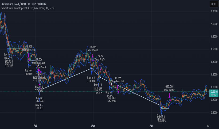
Machine Learning Moving Average [LuxAlgo]The Machine Learning Moving Average (MLMA) is a responsive moving average making use of the weighting function obtained Gaussian Process Regression method. Characteristic such as responsiveness and smoothness can be adjusted by the user from the settings.
The moving average also includes bands, used to highlight possible reversals.
🔶 USAGE
The Machine Learning Moving Average smooths out noisy variations from the price, directly estimating the underlying trend in the price.
A higher "Window" setting will return a longer-term moving average while increasing the "Forecast" setting will affect the responsiveness and smoothness of the moving average, with higher positive values returning a more responsive moving average and negative values returning a smoother but less responsive moving average.
Do note that an excessively high "Forecast" setting will result in overshoots, with the moving average having a poor fit with the price.
The moving average color is determined according to the estimated trend direction based on the bands described below, shifting to blue (default) in an uptrend and fushia (default) in downtrends.
The upper and lower extremities represent the range within which price movements likely fluctuate.
Signals are generated when the price crosses above or below the band extremities, with turning points being highlighted by colored circles on the chart.
🔶 SETTINGS
Window: Calculation period of the moving average. Higher values yield a smoother average, emphasizing long-term trends and filtering out short-term fluctuations.
Forecast: Sets the projection horizon for Gaussian Process Regression. Higher values create a more responsive moving average but will result in more overshoots, potentially worsening the fit with the price. Negative values will result in a smoother moving average.
Sigma: Controls the standard deviation of the Gaussian kernel, influencing weight distribution. Higher Sigma values return a longer-term moving average.
Multiplicative Factor: Adjusts the upper and lower extremity bounds, with higher values widening the bands and lowering the amount of returned turning points.
🔶 RELATED SCRIPTS
Machine-Learning-Gaussian-Process-Regression
SuperTrend-AI-Clustering
อินดิเคเตอร์
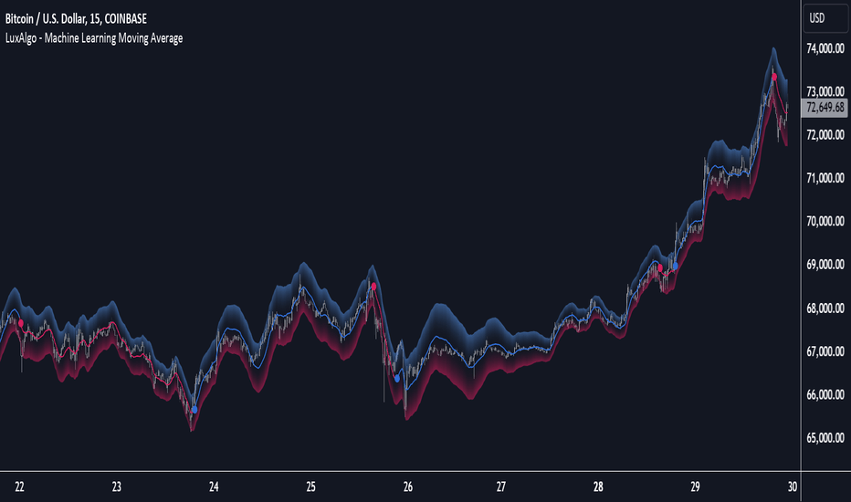
FVG Channel [LuxAlgo]The FVG Channel indicator displays a channel constructed from the averages of unmitigated historical fair value gaps (FVG), allowing to identify trends and potential reversals in the market.
Users can control the amount of FVGs to consider for the calculation of the channels, as well as their degree of smoothness through user settings.
🔶 USAGE
The FVG Channel is constructed by averaging together recent unmitigated Bullish FVGs (contributing to the creation of the upper bands), and Bearish unmitigated FVGs (contributing to the creation of the lower bands) within a lookback determined by the user. A higher lookback will return longer-term indications from the indicator.
The channel includes 5 bands, with one upper and one lower outer extremities, as well as an inner series of values determined using the Fibonacci ratios (respectively 0.786, 0.5, 0.236) from the channel's outer extremities.
An uptrend can be identified by price holding above the inner upper band (obtained from the 0.786 ratio), this band can also provide occasional support when the price retraces to it while in an uptrend.
Breaking below the inner upper band with an unwillingness to reach above again is a clear sign of hesitation in the market and can be indicative of an upcoming consolidation or reversal.
This can directly be applied to downtrends as well, below are examples displaying both scenarios.
Uptrend Example:
Downtrend Example:
🔹 Breakout Levels
When the price mitigates all FVGs in a single direction except for 1, the indicator will display a "Breakout Level". This is the level that price will need to cross in order for all FVGs in that direction to be mitigated, because of this they can also be aptly called "Last Stand Levels".
These levels can be considered as potential support and resistance levels, however, should always be monitored for breakouts since a substantial push above or below these points would indicate strong momentum.
🔹 Signals
The indicator includes Bullish and Bearish Signals, these signals fire when all FVGs for a single direction have been mitigated and an engulfing candle occurs in the opposite direction. These are reversal signals and should be used alongside other indicators to appropriately manage risk.
Note: When all FVGs in a single direction have been mitigated, the candles will change colors accordingly.
🔶 DETAILS
The script uses a typical identification method for FVGs. Once identified, the script collects and stores the mitigation levels of the respective bullish and bearish FVGs:
For Bullish FVGs this is the bottom of the FVG.
For Bearish FVGs this is the top of the FVG.
The data is managed to only consider a specific amount of FVG mitigation levels, determined by the set "Unmitigated FVG Lookback". If an FVG is mitigated, it frees up a spot in the memory for a new FVG, however, if the memory is full, the oldest will be deleted.
The averages displayed (Channel Upper and Lower) are created from 2 calculation steps, the first step involves taking the raw average of the FVG mitigation levels, and the second step applies a simple moving average (SMA) smoothing of the precedent obtained averages.
Note: To view the mitigation levels average obtained in the first step, the "Smoothing Length" can be set to 1.
🔶 SETTINGS
Unmitigated FVG Lookback: Sets the maximum number of Unmitigated FVG mitigation levels that the script will use to calculate the channel.
Smoothing Length: Sets the smoothing length for the channel to reduce noise from the raw data.
อินดิเคเตอร์
Sinc Bollinger BandsKaiser Windowed Sinc Bollinger Bands Indicator
The Kaiser Windowed Sinc Bollinger Bands indicator combines the advanced filtering capabilities of the Kaiser Windowed Sinc Moving Average with the volatility measurement of Bollinger Bands. This indicator represents a sophisticated approach to trend identification and volatility analysis in financial markets.
Core Components
At the heart of this indicator is the Kaiser Windowed Sinc Moving Average, which utilizes the sinc function as an ideal low-pass filter, windowed by the Kaiser function. This combination allows for precise control over the frequency response of the moving average, effectively separating trend from noise in price data.
The sinc function, representing an ideal low-pass filter, provides the foundation for the moving average calculation. By using the sinc function, analysts can independently control two critical parameters: the cutoff frequency and the number of samples used. The cutoff frequency determines which price movements are considered significant (low frequency) and which are treated as noise (high frequency). The number of samples influences the filter's accuracy and steepness, allowing for a more precise approximation of the ideal low-pass filter without altering its fundamental frequency response characteristics.
The Kaiser window is applied to the sinc function to create a practical, finite-length filter while minimizing unwanted oscillations in the frequency domain. The alpha parameter of the Kaiser window allows users to fine-tune the trade-off between the main-lobe width and side-lobe levels in the frequency response.
Bollinger Bands Implementation
Building upon the Kaiser Windowed Sinc Moving Average, this indicator adds Bollinger Bands to provide a measure of price volatility. The bands are calculated by adding and subtracting a multiple of the standard deviation from the moving average.
Advanced Centered Standard Deviation Calculation
A unique feature of this indicator is its specialized standard deviation calculation for the centered mode. This method employs the Kaiser window to create a smooth deviation that serves as an highly effective envelope, even though it's always based on past data.
The centered standard deviation calculation works as follows:
It determines the effective sample size of the Kaiser window.
The window size is then adjusted to reflect the target sample size.
The source data is offset in the calculation to allow for proper centering.
This approach results in a highly accurate and smooth volatility estimation. The centered standard deviation provides a more refined and responsive measure of price volatility compared to traditional methods, particularly useful for historical analysis and backtesting.
Operational Modes
The indicator offers two operational modes:
Non-Centered (Real-time) Mode: Uses half of the windowed sinc function and a traditional standard deviation calculation. This mode is suitable for real-time analysis and current market conditions.
Centered Mode: Utilizes the full windowed sinc function and the specialized Kaiser window-based standard deviation calculation. While this mode introduces a delay, it offers the most accurate trend and volatility identification for historical analysis.
Customizable Parameters
The Kaiser Windowed Sinc Bollinger Bands indicator provides several key parameters for customization:
Cutoff: Controls the filter's cutoff frequency, determining the divide between trends and noise.
Number of Samples: Sets the number of samples used in the FIR filter calculation, affecting the filter's accuracy and computational complexity.
Alpha: Influences the shape of the Kaiser window, allowing for fine-tuning of the filter's frequency response characteristics.
Standard Deviation Length: Determines the period over which volatility is calculated.
Multiplier: Sets the number of standard deviations used for the Bollinger Bands.
Centered Alpha: Specific to the centered mode, this parameter affects the Kaiser window used in the specialized standard deviation calculation.
Visualization Features
To enhance the analytical value of the indicator, several visualization options are included:
Gradient Coloring: Offers a range of color schemes to represent trend direction and strength for the moving average line.
Glow Effect: An optional visual enhancement for improved line visibility.
Background Fill: Highlights the area between the Bollinger Bands, aiding in volatility visualization.
Applications in Technical Analysis
The Kaiser Windowed Sinc Bollinger Bands indicator is particularly useful for:
Precise trend identification with reduced noise influence
Advanced volatility analysis, especially in the centered mode
Identifying potential overbought and oversold conditions
Recognizing periods of price consolidation and potential breakouts
Compared to traditional Bollinger Bands, this indicator offers superior frequency response characteristics in its moving average and a more refined volatility measurement, especially in centered mode. These features allow for a more nuanced analysis of price trends and volatility patterns across various market conditions and timeframes.
Conclusion
The Kaiser Windowed Sinc Bollinger Bands indicator represents a significant advancement in technical analysis tools. By combining the ideal low-pass filter characteristics of the sinc function, the practical benefits of Kaiser windowing, and an innovative approach to volatility measurement, this indicator provides traders and analysts with a sophisticated instrument for examining price trends and market volatility.
Its implementation in Pine Script contributes to the TradingView community by making advanced signal processing and statistical techniques accessible for experimentation and further development in technical analysis. This indicator serves not only as a practical tool for market analysis but also as an educational resource for those interested in the intersection of signal processing, statistics, and financial markets.
Related:
อินดิเคเตอร์