Güncellendi
Nasan Multi-Stage Analog Forecast Model
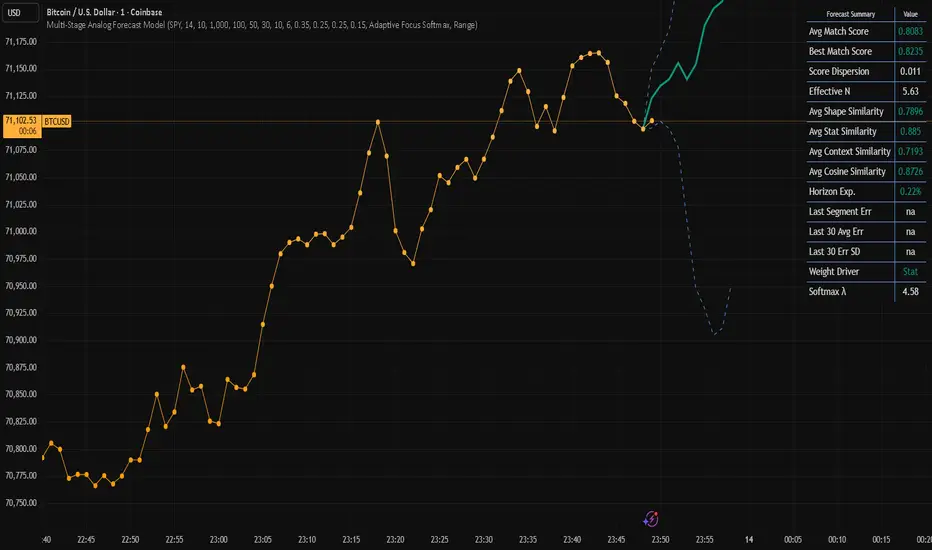
Multi-Stage Analog Forecast Model
The Multi-Stage Analog Forecast Model is a historical pattern-matching forecasting engine that searches past market data for segments that resemble the current market environment. Instead of relying on a single technical indicator, the model compares price shape, statistical structure, market regime, and internal market flow to identify the most relevant historical analogs.
The future behavior of those analog segments is then combined to produce a probabilistic price projection.
Core Idea
Markets often repeat structural conditions rather than exact prices.
If a current market segment resembles a past segment in terms of pattern, volatility structure, momentum state, and internal flow dynamics, the forward behavior of that past segment may provide a useful guide to what could happen next.
To identify these situations, the model applies a four-stage filtering process.
Stage 1 — Pattern Shape Similarity
The first stage compares the shape of the current price segment with historical segments.
Each segment is normalized using Min-Max scaling:
x_norm = (x − min(x)) / (max(x) − min(x))
This removes the effect of price level so that patterns can be compared regardless of whether the asset was trading at $50 or $500.
Similarity is measured using Euclidean distance:
Distance = sqrt( Σ (Current_i − Historical_i)^2 )
Segments with the smallest distances represent the closest geometric matches.
Stage 2 — Statistical Similarity
The second stage checks whether the statistical structure of the move matches.
Price is standardized using a lagged normalization:
Z = (Price − SMA_prev) / StDev_prev
where the mean and standard deviation are shifted one bar back.
This produces a one-bar-lagged standardized deviation, measuring how extreme the move is relative to the previous volatility environment.
Segments are compared using Spearman rank correlation:
ρ = corr(rank(Z_current), rank(Z_historical))
This ensures the internal statistical rhythm of the move is similar.
Stage 3 — Market Context Filter (APD)
Even if two patterns look similar, they may occur in very different market environments.
The third stage evaluates context similarity using Average Percentage Distance (APD) across eight factors:
Volatility regime: VolRegime = ATR(14) / ATR(55)
Momentum: RSI(14)
Volume participation: VolPart = Volume / SMA(Volume,55)
Trend velocity: TrendMove = (EMA14 − EMA14[segLen]) / ATR14
Trend stretch:TrendStretch = (EMA14 − Price) / ATR14
Relative strength vs benchmark
Structural trend spread: (EMA200 − EMA50) / ATR
Intermediate trend spread: (EMA50 − EMA21) / ATR
Differences are measured using symmetric percentage distance:
SPD(a,b) = |a − b| / max(|a|, |b|)
The overall context mismatch is:
APD = average(SPD values)
Lower APD means the historical segment occurred in a similar market regime.
Stage 4 — Structural Flow Similarity
The fourth stage compares the internal market engine using cosine similarity.
Five flow signals are constructed:
Sentiment flow (signed volume pressure)
Volatility flow: ATR(14)
Noise flow: StDev(TrueRange)
Structure flow: (EMA13 − EMA34) / ATR
Momentum flow: RSI(14)
Each signal is converted into a segment flow measure:
Flow = average( x − x[i+1] )
These flows form a vector:
V = (v1, v2, v3, v4, v5)
Similarity between current and historical vectors is measured using cosine similarity:
CosSim = (A · B) / (|A| |B|)
Higher cosine similarity means the internal market forces are aligned.
Final Analog Score
Each candidate receives a composite score combining the four stages:
Score =wShape * ShapeSim + wStat * StatSim + wCtx * ContextSim + wCos * CosSim
The highest scoring segments become the final analog set.
Forecast Construction
For each analog segment, the model calculates forward returns:
Return_h = (FuturePrice / SegmentEndPrice) − 1
The expected return at step h is the weighted average:
μ_h = Σ (Weight_i × Return_i,h)
Projected price:
Forecast = CurrentPrice × (1 + μ_h)
Dispersion among analog outcomes is measured as:
σ_h = sqrt( Σ Weight_i × (Return_i,h − μ_h)^2 )
Upper and lower forecast bands are:
Upper = P0 × (1 + μ_h + σ_h)
Lower = P0 × (1 + μ_h − σ_h)
Forecast Error Measurement
The model also tracks how accurate its past forecasts were.
Prediction error is measured in volatility-adjusted units:
Error = |Predicted − Actual| / (ATR(55) × √h)
ATR(55) normalizes the error to volatility units so it is comparable across assets and regimes.
The √h term accounts for the fact that uncertainty grows with forecast horizon.
Recent forecast errors are averaged to provide a real-time model reliability diagnostic.
How to Interpret the Forecast
• The solid line represents the expected price path based on historical analogs.
• The dashed bands represent dispersion among those analog outcomes.
Narrow bands indicate stronger agreement between historical cases, while wider bands suggest lower certainty.
Because the model is based on historical analogs rather than deterministic rules, it should be interpreted as a probabilistic guide to potential market direction.
The Multi-Stage Analog Forecast Model is a historical pattern-matching forecasting engine that searches past market data for segments that resemble the current market environment. Instead of relying on a single technical indicator, the model compares price shape, statistical structure, market regime, and internal market flow to identify the most relevant historical analogs.
The future behavior of those analog segments is then combined to produce a probabilistic price projection.
Core Idea
Markets often repeat structural conditions rather than exact prices.
If a current market segment resembles a past segment in terms of pattern, volatility structure, momentum state, and internal flow dynamics, the forward behavior of that past segment may provide a useful guide to what could happen next.
To identify these situations, the model applies a four-stage filtering process.
Stage 1 — Pattern Shape Similarity
The first stage compares the shape of the current price segment with historical segments.
Each segment is normalized using Min-Max scaling:
x_norm = (x − min(x)) / (max(x) − min(x))
This removes the effect of price level so that patterns can be compared regardless of whether the asset was trading at $50 or $500.
Similarity is measured using Euclidean distance:
Distance = sqrt( Σ (Current_i − Historical_i)^2 )
Segments with the smallest distances represent the closest geometric matches.
Stage 2 — Statistical Similarity
The second stage checks whether the statistical structure of the move matches.
Price is standardized using a lagged normalization:
Z = (Price − SMA_prev) / StDev_prev
where the mean and standard deviation are shifted one bar back.
This produces a one-bar-lagged standardized deviation, measuring how extreme the move is relative to the previous volatility environment.
Segments are compared using Spearman rank correlation:
ρ = corr(rank(Z_current), rank(Z_historical))
This ensures the internal statistical rhythm of the move is similar.
Stage 3 — Market Context Filter (APD)
Even if two patterns look similar, they may occur in very different market environments.
The third stage evaluates context similarity using Average Percentage Distance (APD) across eight factors:
Volatility regime: VolRegime = ATR(14) / ATR(55)
Momentum: RSI(14)
Volume participation: VolPart = Volume / SMA(Volume,55)
Trend velocity: TrendMove = (EMA14 − EMA14[segLen]) / ATR14
Trend stretch:TrendStretch = (EMA14 − Price) / ATR14
Relative strength vs benchmark
Structural trend spread: (EMA200 − EMA50) / ATR
Intermediate trend spread: (EMA50 − EMA21) / ATR
Differences are measured using symmetric percentage distance:
SPD(a,b) = |a − b| / max(|a|, |b|)
The overall context mismatch is:
APD = average(SPD values)
Lower APD means the historical segment occurred in a similar market regime.
Stage 4 — Structural Flow Similarity
The fourth stage compares the internal market engine using cosine similarity.
Five flow signals are constructed:
Sentiment flow (signed volume pressure)
Volatility flow: ATR(14)
Noise flow: StDev(TrueRange)
Structure flow: (EMA13 − EMA34) / ATR
Momentum flow: RSI(14)
Each signal is converted into a segment flow measure:
Flow = average( x − x[i+1] )
These flows form a vector:
V = (v1, v2, v3, v4, v5)
Similarity between current and historical vectors is measured using cosine similarity:
CosSim = (A · B) / (|A| |B|)
Higher cosine similarity means the internal market forces are aligned.
Final Analog Score
Each candidate receives a composite score combining the four stages:
Score =wShape * ShapeSim + wStat * StatSim + wCtx * ContextSim + wCos * CosSim
The highest scoring segments become the final analog set.
Forecast Construction
For each analog segment, the model calculates forward returns:
Return_h = (FuturePrice / SegmentEndPrice) − 1
The expected return at step h is the weighted average:
μ_h = Σ (Weight_i × Return_i,h)
Projected price:
Forecast = CurrentPrice × (1 + μ_h)
Dispersion among analog outcomes is measured as:
σ_h = sqrt( Σ Weight_i × (Return_i,h − μ_h)^2 )
Upper and lower forecast bands are:
Upper = P0 × (1 + μ_h + σ_h)
Lower = P0 × (1 + μ_h − σ_h)
Forecast Error Measurement
The model also tracks how accurate its past forecasts were.
Prediction error is measured in volatility-adjusted units:
Error = |Predicted − Actual| / (ATR(55) × √h)
ATR(55) normalizes the error to volatility units so it is comparable across assets and regimes.
The √h term accounts for the fact that uncertainty grows with forecast horizon.
Recent forecast errors are averaged to provide a real-time model reliability diagnostic.
How to Interpret the Forecast
• The solid line represents the expected price path based on historical analogs.
• The dashed bands represent dispersion among those analog outcomes.
Narrow bands indicate stronger agreement between historical cases, while wider bands suggest lower certainty.
Because the model is based on historical analogs rather than deterministic rules, it should be interpreted as a probabilistic guide to potential market direction.
Sürüm Notları
This revision introduces Adaptive Focus Softmax weighting and stabilizes the analog selection process. Previously, linear weights were used to combine analog outcomes; this update replaces that approach with probabilistic softmax weighting.Final analogs are now strictly selected using the composite similarity score (Shape, Statistical, Context/APD, and Cosine). Once the top N analogs are frozen, their diagnostic statistics (average score, score dispersion, and similarity metrics) remain fixed and are no longer affected by forecast weighting changes.
The forecast itself is then produced using adaptive softmax weighting. The model evaluates the dispersion of the four similarity stages among the final analogs and automatically selects the stage with the highest variability (measured by CV or Range) as the weighting driver. This allows the forecast to emphasize the similarity dimension that currently provides the strongest discrimination between analog candidates.
Analog weights are computed using the softmax (Gibbs) distribution:
wᵢ = exp(λ · sᵢ) / Σ exp(λ · sⱼ)
where
sᵢ = similarity score of analog i
wᵢ = resulting weight
λ = concentration parameter.
Softmax pressure is now determined automatically using
λ = 2 · ln(N) + 1
where N is the number of final analogs. This scaling provides stable weighting across different analog pool sizes without relying on unstable score-dispersion formulas.
The same weights are used consistently for both the weighted forecast mean and the weighted variance, ensuring that the forecast bands reflect the similarity-weighted dispersion of the analog outcomes.
Sürüm Notları
Chart fix
Feragatname
Bilgiler ve yayınlar, TradingView tarafından sağlanan veya onaylanan finansal, yatırım, alım satım veya diğer türden tavsiye veya öneriler anlamına gelmez ve teşkil etmez. Kullanım Koşulları bölümünde daha fazlasını okuyun.
Feragatname
Bilgiler ve yayınlar, TradingView tarafından sağlanan veya onaylanan finansal, yatırım, alım satım veya diğer türden tavsiye veya öneriler anlamına gelmez ve teşkil etmez. Kullanım Koşulları bölümünde daha fazlasını okuyun.