State-Dependent EMA [BackQuant]
More exclusive indicators from BackQuant
Subscribe to Trading & Portfolio Toolkit for $69.99/month to get exclusive indicators by this author. You pay right on TradingView and can use them on your charts straight away.
Explore Trading & Portfolio ToolkitState-Dependent EMA [BackQuant]
Overview
State-Dependent EMA is an adaptive exponential moving average that adjusts its smoothing coefficient using three measurements: price efficiency, sustained deviation from the filter, and changes in short-term volatility.
Rather than using a fixed EMA length, the indicator calculates a smoothing coefficient between the selected Fast and Slow EMA settings. The coefficient changes as the estimated market state changes, allowing the filter to respond more quickly under some conditions and apply greater smoothing under others.
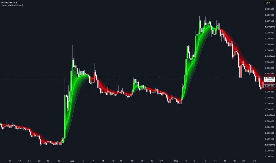
The indicator includes three state models, an optional volatility penalty, two methods of determining trend direction, a gradient ribbon and a fixed EMA for comparison.
Core Calculation
The filter uses the standard recursive EMA update:
Filter = Previous Filter + Alpha × (Source - Previous Filter)
The difference is that Alpha is recalculated on every bar rather than remaining fixed.
The adaptive coefficient is calculated as:
Alpha = Slow Alpha + (Fast Alpha - Slow Alpha) × Market State
Market State ranges from 0 to 1.
Fast and Slow EMA Length define the coefficient limits. The script does not blend two separately calculated EMA lines.
State Estimation
Three state models are available: Efficiency, Sustained Residual and Combined. All three can be moderated by the optional variance penalty.
Efficiency
The efficiency calculation compares net price displacement with the total absolute movement over the selected Efficiency Length.
Efficiency = |Source - Source[N]| / Sum of Absolute Bar-to-Bar Changes
The result ranges from 0 to 1.
A value near 1 indicates that most movement over the window occurred in one direction. A value near 0 indicates that price travelled considerably more than its final net displacement.
High efficiency increases the adaptive coefficient, while low efficiency favours greater smoothing.
The calculation measures directional efficiency regardless of whether price is rising or falling.
Sustained Residual
The residual model measures how far the current Source is from the previous filtered value:
Innovation = Source - Previous Filter
This difference is smoothed using an EMA over the selected Residual Persistence length. Its absolute value is then divided by ATR and scaled using Residual Scale.
The result is capped at 1.
This allows the filter to increase its response when the Source remains displaced from its previous estimate.
The absolute residual is used, so upward and downward deviations are treated equally. The residual state controls responsiveness, not bullish or bearish direction.
Combined State
Combined mode blends the Efficiency and Sustained Residual states using the two configurable weights.
Combined State = (Efficiency × Efficiency Weight + Residual State × Residual Weight) / Total Weight
The weights are normalized by their sum, so they determine the relative contribution of each component.
If both weights are zero, the combined state is zero.
Variance Penalty
The indicator compares the short-term and long-term standard deviations of one-bar Source changes.
Despite the input's name, the calculated Variance Ratio is a ratio of standard deviations, not a ratio of squared variances.
When short-term volatility exceeds its longer-term baseline, the variance penalty can reduce the calculated state:
Variance Gate = 1 / (1 + Penalty × max(Volatility Ratio - 1, 0))
The selected state is multiplied by this gate before the adaptive Alpha is calculated.
This means an increase in efficiency or sustained residual does not always produce a faster filter. A simultaneous increase in short-term volatility can partially offset it.
Set Variance Penalty to 0 to disable this adjustment.
Trend Direction
Two trend methods are available.
Ribbon
Compares the adaptive filter with an EMA of its own values over the selected Ribbon Length.
Filter Slope
Compares the current filtered value with its value at the selected Slope Lookback.
In either mode, an exact equality retains the previous trend state.
The selected trend method controls line colour, optional candle and background colouring, and bullish/bearish alerts.
Visuals
The Gradient Ribbon displays the distance between the adaptive filter and its smoothed reference.
The optional Price Gradient fills the area between the filter and the chart's closing price. This uses Close even when a different calculation Source is selected.
Filter Glow adds an ATR-scaled visual band around the adaptive line. It does not affect the state estimation or trend signals.
The Fixed EMA Comparison plots a conventional EMA of the selected Source, making it possible to compare the adaptive response against a fixed-length smoother.
Input Guide
Data Window
The Data Window exposes the current Adaptive Alpha, Effective EMA Length, Efficiency Ratio, Sustained Residual State, Variance Ratio and final Market State.
Effective EMA Length is calculated as:
Effective Length = 2 / Alpha - 1
This expresses the current smoothing coefficient as an equivalent fixed EMA length. Because Alpha changes through time, it is not the length of a single fixed-window calculation.
These values are useful when comparing how the different state models and variance settings affect the filter.
Limitations
The state measurements are based on current and historical data. They do not predict future price direction.
High efficiency can occur in either rising or falling markets. Likewise, a large sustained residual can increase responsiveness in either direction.
The variance penalty can reduce responsiveness during periods of increased short-term volatility, including genuine directional moves. More aggressive settings may respond faster but can also introduce more frequent changes in trend colour.
As with other moving averages, the indicator remains sensitive to its selected lengths and can produce repeated trend changes in sideways conditions.
Alerts
Summary
State-Dependent EMA adjusts a standard EMA smoothing coefficient using price efficiency, sustained deviation from the previous filtered value, or a combination of both. An optional volatility penalty moderates the response when short-term price-change volatility rises above its longer-term baseline.
The resulting line can be evaluated using either a smoothed ribbon or its own slope, with a fixed EMA comparison and Data Window measurements available for inspecting how the adaptive settings affect its behaviour.
Overview
State-Dependent EMA is an adaptive exponential moving average that adjusts its smoothing coefficient using three measurements: price efficiency, sustained deviation from the filter, and changes in short-term volatility.
Rather than using a fixed EMA length, the indicator calculates a smoothing coefficient between the selected Fast and Slow EMA settings. The coefficient changes as the estimated market state changes, allowing the filter to respond more quickly under some conditions and apply greater smoothing under others.
The indicator includes three state models, an optional volatility penalty, two methods of determining trend direction, a gradient ribbon and a fixed EMA for comparison.
Core Calculation
The filter uses the standard recursive EMA update:
Filter = Previous Filter + Alpha × (Source - Previous Filter)
The difference is that Alpha is recalculated on every bar rather than remaining fixed.
The adaptive coefficient is calculated as:
Alpha = Slow Alpha + (Fast Alpha - Slow Alpha) × Market State
Market State ranges from 0 to 1.
- A state near 0 produces a coefficient close to the Slow EMA setting.
- A state near 1 produces a coefficient close to the Fast EMA setting.
- Intermediate values produce a response between the two.
Fast and Slow EMA Length define the coefficient limits. The script does not blend two separately calculated EMA lines.
State Estimation
Three state models are available: Efficiency, Sustained Residual and Combined. All three can be moderated by the optional variance penalty.
Efficiency
The efficiency calculation compares net price displacement with the total absolute movement over the selected Efficiency Length.
Efficiency = |Source - Source[N]| / Sum of Absolute Bar-to-Bar Changes
The result ranges from 0 to 1.
A value near 1 indicates that most movement over the window occurred in one direction. A value near 0 indicates that price travelled considerably more than its final net displacement.
High efficiency increases the adaptive coefficient, while low efficiency favours greater smoothing.
The calculation measures directional efficiency regardless of whether price is rising or falling.
Sustained Residual
The residual model measures how far the current Source is from the previous filtered value:
Innovation = Source - Previous Filter
This difference is smoothed using an EMA over the selected Residual Persistence length. Its absolute value is then divided by ATR and scaled using Residual Scale.
The result is capped at 1.
- A small or inconsistent residual produces a lower state value.
- A larger residual that persists in one direction produces a higher state value.
This allows the filter to increase its response when the Source remains displaced from its previous estimate.
The absolute residual is used, so upward and downward deviations are treated equally. The residual state controls responsiveness, not bullish or bearish direction.
Combined State
Combined mode blends the Efficiency and Sustained Residual states using the two configurable weights.
Combined State = (Efficiency × Efficiency Weight + Residual State × Residual Weight) / Total Weight
The weights are normalized by their sum, so they determine the relative contribution of each component.
If both weights are zero, the combined state is zero.
Variance Penalty
The indicator compares the short-term and long-term standard deviations of one-bar Source changes.
Despite the input's name, the calculated Variance Ratio is a ratio of standard deviations, not a ratio of squared variances.
When short-term volatility exceeds its longer-term baseline, the variance penalty can reduce the calculated state:
Variance Gate = 1 / (1 + Penalty × max(Volatility Ratio - 1, 0))
The selected state is multiplied by this gate before the adaptive Alpha is calculated.
This means an increase in efficiency or sustained residual does not always produce a faster filter. A simultaneous increase in short-term volatility can partially offset it.
Set Variance Penalty to 0 to disable this adjustment.
Trend Direction
Two trend methods are available.
Ribbon
Compares the adaptive filter with an EMA of its own values over the selected Ribbon Length.
- Filter above Ribbon = bullish.
- Filter below Ribbon = bearish.
Filter Slope
Compares the current filtered value with its value at the selected Slope Lookback.
- Filter rising = bullish.
- Filter falling = bearish.
In either mode, an exact equality retains the previous trend state.
The selected trend method controls line colour, optional candle and background colouring, and bullish/bearish alerts.
Visuals
The Gradient Ribbon displays the distance between the adaptive filter and its smoothed reference.
The optional Price Gradient fills the area between the filter and the chart's closing price. This uses Close even when a different calculation Source is selected.
Filter Glow adds an ATR-scaled visual band around the adaptive line. It does not affect the state estimation or trend signals.
The Fixed EMA Comparison plots a conventional EMA of the selected Source, making it possible to compare the adaptive response against a fixed-length smoother.
Input Guide
- Fast / Slow EMA Length: Set the response limits of the adaptive filter.
- State Model: Select Efficiency, Sustained Residual or their weighted combination.
- Efficiency Length: Lookback used to compare net displacement with total movement.
- Residual Persistence: EMA smoothing length applied to the filter's residual.
- ATR Length: Normalization period for the residual state.
- Residual Scale: Controls how much normalized residual is required to reach the maximum residual state.
- Efficiency / Residual Weight: Set the relative contribution of each component in Combined mode.
- Short / Long Variance Length: Define the two standard-deviation windows used by the volatility comparison.
- Variance Penalty: Controls how strongly elevated short-term volatility reduces responsiveness.
- Ribbon Length: Smoothing length for the ribbon reference.
- Trend Direction: Select the Ribbon or Filter Slope method.
- Slope Lookback: Comparison period used by Filter Slope mode.
Data Window
The Data Window exposes the current Adaptive Alpha, Effective EMA Length, Efficiency Ratio, Sustained Residual State, Variance Ratio and final Market State.
Effective EMA Length is calculated as:
Effective Length = 2 / Alpha - 1
This expresses the current smoothing coefficient as an equivalent fixed EMA length. Because Alpha changes through time, it is not the length of a single fixed-window calculation.
These values are useful when comparing how the different state models and variance settings affect the filter.
Limitations
The state measurements are based on current and historical data. They do not predict future price direction.
High efficiency can occur in either rising or falling markets. Likewise, a large sustained residual can increase responsiveness in either direction.
The variance penalty can reduce responsiveness during periods of increased short-term volatility, including genuine directional moves. More aggressive settings may respond faster but can also introduce more frequent changes in trend colour.
As with other moving averages, the indicator remains sensitive to its selected lengths and can produce repeated trend changes in sideways conditions.
Alerts
- State EMA Bullish: the selected trend method changes from bearish to bullish.
- State EMA Bearish: the selected trend method changes from bullish to bearish.
Summary
State-Dependent EMA adjusts a standard EMA smoothing coefficient using price efficiency, sustained deviation from the previous filtered value, or a combination of both. An optional volatility penalty moderates the response when short-term price-change volatility rises above its longer-term baseline.
The resulting line can be evaluated using either a smoothed ribbon or its own slope, with a fixed EMA comparison and Data Window measurements available for inspecting how the adaptive settings affect its behaviour.

Join the Paid Space or get access to my invite only scripts at
backquant.com/
Or join the free discord discord.gg/RmVrJV67yE
backquant.com/
Or join the free discord discord.gg/RmVrJV67yE
Feragatname
Bilgiler ve yayınlar, TradingView tarafından sağlanan veya onaylanan finansal, yatırım, alım satım veya diğer türden tavsiye veya öneriler anlamına gelmez ve teşkil etmez. Kullanım Koşulları bölümünde daha fazlasını okuyun.
Join the Paid Space or get access to my invite only scripts at
backquant.com/
Or join the free discord discord.gg/RmVrJV67yE
backquant.com/
Or join the free discord discord.gg/RmVrJV67yE
Feragatname
Bilgiler ve yayınlar, TradingView tarafından sağlanan veya onaylanan finansal, yatırım, alım satım veya diğer türden tavsiye veya öneriler anlamına gelmez ve teşkil etmez. Kullanım Koşulları bölümünde daha fazlasını okuyun.