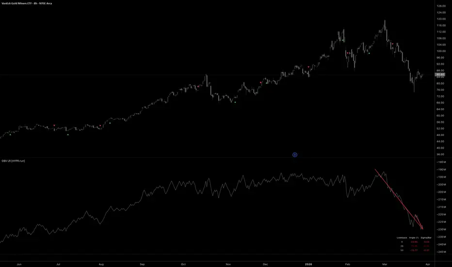
Linear Regression Channel Fit AuditLinear Regression Channel Fit Audit
Overview
Linear Regression Channel Fit Audit is a price-chart overlay for studying statistical slope and the behavior of a rolling regression channel. It separates three questions: how well a line fits its own historical window, how the next observation compares with the model available before it arrived, and what happens when an earlier model is kept unchanged through several later observations.
The practical question is simple: did price fit the channel that was available beforehand, or did updating the channel make it appear to fit?
The script combines a current ordinary least-squares channel, a previous-model reference, refit attribution, historical as-of inspection, and scheduled frozen-channel studies. It is a descriptive model-diagnostics indicator, not a trading strategy, probability forecast, or source of entry and exit instructions.
What distinguishes the approach
Regression lines, residual bands, R-squared and historical channels are established tools. The contribution here is their use in a connected comparison of model updates and subsequent observations.
The same observation is evaluated before and after refitting. Movement of the fitted center is separated into removal of the oldest observation and addition of the newest. Changes in containment are examined separately through center movement and width changes. Earlier models are also retained on a predetermined schedule, allowing endpoint containment to be distinguished from containment throughout the observed path. Matched comparisons then show how a fixed model differs from an updating model and how shifting the starting level affects extrapolation errors.
These components address one problem: a rolling channel can change its apparent relationship with price because the model itself has moved or widened. They do not vote on a combined trade score or choose a supposedly best model.
Getting started
Use standard time-based candles and a price-valued Source. The default Source is close, the regression length is 120 bars, and the width is twice the residual standard error. Snapshot updates default to Confirmed close.
Start with the Model panel. Read the slope and in-window fit, then compare Prior/Now. Use Refit research to examine the effect of updating the model, Horizon research for one-step and H-step endpoint checks, and Frozen paths for complete fixed-model observation sequences.
Historical frozen paths are enabled by default. Four recent paths are retained for display. Each evaluates 24 later Source values, followed by a 24-bar gap, so scheduled origins are 48 bars apart. Drawing retention and numerical sample retention are separate controls.
Chart guide
The solid upper and lower boundaries are cyan and pink by default. The solid center is colored according to rising, falling or approximately flat normalized slope. Optional dotted inner guides and transparent shading help locate price within the selected width. These colors describe geometry, not trade direction.
OLS identifies the fitted center. +1w and -1w identify the selected upper and lower boundaries, where w means one channel half-width, not necessarily one standard deviation. The dashed EXT segment continues the current slope and width geometrically. It is not an uncertainty interval and is not used in any audit statistic.
The short amber reference uses the preceding model and its preceding width. Its endpoint at the displayed observation is the one-step reference. Optional historical reference traces connect those successive one-step centers and boundaries; they are not one permanently fixed channel.
Thin dashed channels identified by F1, F2 and similar labels are scheduled frozen paths. They retain their origin model rather than being refitted with later prices. A dotted vertical line marks the origin. Optional amber connectors show the first observed exit and the distance from the fixed center at the latest evaluated observation.
The Forward only setting shows the observed forward portion. Fit + forward additionally restores the original fitted training segment as faint dotted lines. That training segment became available at its origin, not at each older bar through which it is drawn.
Small event symbols have no filled background:
! means a transition outside the respective previous-model envelope, including a direct switch from one outside side to the other.
↺ means refit inclusion has appeared: outside the previous envelope but inside after refitting.
= means a transition inside the respective previous-model envelope again.
An optional letter mode uses O, R and I. These are state transitions, not buy/sell signals. Each observation uses its own preceding model; an inside-again event does not prove that price crossed back through one unchanged boundary.
Symbols are offset outside nearby candle wicks for readability. Their vertical placement is not an event or execution price. When conditions coincide, refit inclusion takes drawing priority. Marker spacing, count and display-window filters can hide glyphs without removing observations or suppressing the corresponding alert conditions.
Regression and residual width
The script fits a straight line to N consecutive Source observations using equally spaced bar positions. It works in source-price units, not log price or elapsed calendar time. For each observation, its residual is its Source value minus the fitted value at the same position in that window.
Three half-width methods are available:
Residual standard error: multiplier * sqrt(SSE / (N - 2)).
Mean absolute residual: multiplier * mean(abs(residual)).
Residual percentile: the nearest-rank percentile of absolute residuals from the fitted window.
SSE is the sum of squared fitted residuals. The percentile method does not use the multiplier. Mean absolute residual is not median absolute deviation. A configurable minimum width in symbol ticks, together with a small numerical floor, prevents a zero denominator on flat or nearly exact-line data. The floor can dominate such samples.
These are descriptive residual envelopes. A selected percentile measures the fitting sample; it does not specify a future coverage probability. None of the methods constructs a confidence interval or prediction interval.
Model panel
Slope is the fitted price change over the selected measurement span divided by the current half-width. The default span is 20 bars. Arrows and the flat threshold use this normalized value. Changing the width method or multiplier can therefore change the normalized slope and its flat classification. It is not an on-screen angle or annualized return.
R-squared measures in-window fit relative to variation around the sample mean. The five-segment meter is a coarse visual representation of that number. Constant data display n/a. High R-squared does not establish useful future prediction.
In/Next compares current fitted-window containment with realized one-step containment over the audit sample. These are different samples. Amber highlights the configured coverage gap after enough valid observations are available; it is not a significance test.
Prior/Now shows the signed Source distance before and after refitting. Prior uses the old half-width; Now uses the new half-width. Values beyond +1 or -1 are outside the respective envelope. Do not subtract these readings as raw price distances because their denominators differ.
Add/Drop reports the center-update components explained below. State refers to the previous envelope, except REFIT IN, which explicitly identifies inclusion after updating. Audit shows the valid observation count. A check mark means the sample is full, not that the model passed a performance test.
Detailed mode also shows one-step error skill, residual persistence, older/recent half-window slopes, width change and the number of refit-included observations. Residual persistence is the sum of adjacent residual products divided by SSE, not a significance test. The two half-window slopes use a common full-channel width; with odd lengths the older half contains one extra observation.
Add/Drop: why the center changed
The previous and current N-observation windows share N - 1 observations. All three models below are evaluated at the current observation's time coordinate:
Previous center: the preceding N-observation model extended by one bar.
Common center: the model fitted to the N - 1 shared observations.
Current center: the newly fitted N-observation model.
Drop = Common center - Previous center.
Add = Current center - Common center.
Add + Drop = Current center - Previous center.
The defined update order removes the oldest observation first and then adds the newest. The calculation uses the least-squares endpoint leverage identity to obtain the addition term without fitting another model on every bar.
Both displayed components are signed shifts in prior half-widths, not percentages. Opposite signs indicate offsetting effects. This is an attribution of a model update, not an explanation of the economic cause of a price movement.
Refit research: center versus width
Before/After compares exactly the same confirmed observations against their respective prior and refitted envelopes. In/Out n counts outside-to-inside and inside-to-outside observations. Their difference accounts for the change in matched containment:
After coverage - Before coverage = (Included observations - Excluded observations) / Paired observations.
The After result includes each observation in its own fit and is not an out-of-sample forecast.
Containment margin is half-width minus the absolute distance from the center. Its change is split into:
Center contribution = abs(old residual) - abs(new residual).
Width contribution = new half-width - old half-width.
Both displayed contributions are divided by the prior half-width, and their sum equals the normalized margin change.
For outside-to-inside observations, the Cause field tests two alternative geometries: new center with old width, and old center with new width.
CENTER: only the center change alone is sufficient.
WIDTH: only the width change alone is sufficient.
JOINT: neither change alone is sufficient; both are needed.
EITHER: either change alone is sufficient.
The four classification counts sum to the included count. These are geometric comparisons, not evidence of price reversal or economic causality. For example, WIDTH can identify a point accommodated by a wider envelope without needing the center to move.
One-step and H-step endpoint research
At observation t, the one-step reference is the center fitted at t-1 plus that model's slope. Its width is the width fitted at t-1. The observation at t is not included in that reference.
The second reference uses the model fitted H bars earlier, extended by H bars while keeping its origin width. H defaults to 5 and is selectable from 2 to 50. Results enter the statistics only when their endpoint has been reached and confirmed. This endpoint test does not require all intermediate observations to remain inside; the Frozen paths study addresses that separate question.
Each horizon reports realized containment and an error-skill comparison with holding its origin Source value unchanged:
Skill (%) = 100 * (1 - Model squared-error sum / Unchanged-source squared-error sum).
Model and baseline use identical eligible observations at that horizon. Positive values mean lower squared error than that baseline; negative values mean higher squared error. A zero baseline error produces n/a. Scores are not returns, win rates or significance levels. The two horizons can have different valid counts and are not necessarily identical samples across horizons.
The page also reports H-step mean absolute error in source-price units, the matching baseline error, mean absolute error normalized by origin width, and upper/lower endpoint misses. Successive horizon tests can overlap and are dependent.
Scheduled frozen paths
A path saves the fitted center, slope, width and Source value at its origin. It then evaluates the next L confirmed Source values without changing those saved parameters:
Fixed center at age k = Origin fitted center + Origin slope * k.
Fixed boundaries = Fixed center at age k +/- Origin half-width.
The origin observation itself is not one of the L tested outcomes. A path is extended only through observations already reached. It is not reset or discarded when price exits. Historical line colors do not change retrospectively to label the whole path as successful or unsuccessful.
Origins follow a bar-count schedule beginning at the first loaded confirmed close at or after Path schedule anchor. They recur every L plus Gap bars. Price behavior does not choose the scheduled times. An invalid origin fit is skipped, not moved to a more favorable observation. Skipped origins are reported in the sample tooltip.
With a zero gap, a path finishes before the next starts on the same close. Tested outcome segments do not overlap, although training windows can overlap and market observations remain dependent.
At maturity, the result label is:
ALL: all L sampled Source values were inside.
BACK: the final Source value was inside after at least one earlier sampled exit.
OUT: the final Source value was outside.
DATA: the path contained missing Source observations and is excluded from valid-result denominators.
A fraction such as 8/24 indicates an unfinished path. It is not counted as success or failure. ALL is about sampled Source values at confirmed bars, not an intrabar high/low test. With close as Source, a wick can exceed a boundary while the sampled close remains inside.
The first-exit connector marks the first observed outside Source value, not an intrabar crossing or order fill. Maximum distance is the largest sampled absolute distance from the fixed center divided by origin width.
For a simple example, a path that exits at age 6 and finishes inside at age 24 is BACK, not ALL. Looking only at the final observation would miss that distinction.
Frozen paths panel and matched comparisons
End/All reports final-observation containment and every-observation containment over the same valid completed paths. Back/Exit reports paths ending inside after an exit and paths with any sampled exit. End count equals All count plus Back count.
First exit is the average first-exit age among exited, valid, completed paths only. Paths without an exit and unfinished paths are not assigned zero-time exits. This conditional average is not a survival estimate.
F/A skill compares two centers against one common unchanged-origin-Source baseline over the same complete paths:
F: origin fitted center + origin slope * k.
A: origin Source + the same origin slope * k.
A changes the starting level, not the slope. The comparison helps inspect the effect of initial fitted-center displacement. It does not prove that the slope is useful or select a winning model. Scores use pooled squared errors across all included observations, not an average of individual path percentages.
Roll/Fix compares updating one-step envelopes with the saved fixed envelope on the same eligible observations within valid completed paths. It reports the percentage inside only the updating envelope and the percentage inside only the fixed envelope. Both-inside and both-outside counts are also available in the tooltip, along with matched error comparisons.
Both references exclude the observation being tested, but the updating model has intermediate information that the fixed model does not. Their widths may also differ. This comparison measures the effect of updating; it is not a contest between models with equal information.
Paired gives the number of matched observations. Done/Open gives the valid completed-path count and current unfinished age. Missing-data slots are separately disclosed and remain part of slot retention. The drawing cap never changes the numerical sample.
As-of research and sample scope
Set View to As-of research, choose Research start and As-of cutoff, and select the relevant panel page. The main channel and snapshot represent the last available confirmed bar whose close time is inside that interval. The header or its tooltip identifies the actual selected close in the exchange timezone.
Training can use earlier observations, but test origins must be calculated inside the admitted interval. One-step and H-step results therefore need their respective earlier origin models. The script does not invent those initial tests. A frozen path still unfinished at the cutoff remains unfinished.
Rolling audit uses the last K chart bars for the ordinary audit metrics. Selected interval aggregates valid tests admitted throughout the interval. Frozen-path statistics have a separate completed-slot sample: Latest and Rolling research retain up to the configured number of completed slots; Selected interval uses all completed slots. Actual counts, not requested maxima, determine the denominators.
As-of mode does not scroll the chart or hide later candles. It reconstructs the model at the selected time, but it is not a blind replay environment. Alerts are disabled in this mode. Later loaded timestamps can place optional annotations; later Source prices do not enter the selected model or its statistics. Without those timestamps, annotation spacing beyond loaded data uses a nominal bar duration and can differ around session gaps or irregular periods.
Schedule reproducibility and workload
If the path anchor is at or before the beginning of loaded history, the Frozen paths header displays PHASE*. The schedule may then change when additional earlier bars load. For reproducible comparisons, place the anchor within loaded history with earlier bars available, and retain the same symbol, timeframe, settings and research interval.
The default calculation budget is 600 bars, configurable from 100 to 4,000. Latest view adds audit/horizon warm-up to the recent fitted range. Frozen-path origins and retained results are bounded by the recent path range; chronological path IDs are local identifiers, not permanent IDs across recalculations.
In research, the budget is a hard limit on admitted interval bars. RANGE > CAP blocks the main research display rather than silently presenting an earlier endpoint as the selected result. Earlier traces or numeric records can remain partial and must not be read as complete interval results. Narrow the dates or raise the budget. START > END, NO ELIGIBLE BAR and WARM-UP / DATA identify other unavailable states.
Larger windows and percentile sorting increase processing cost. Drawing caps are independent of statistical caps. Up to 12 paths can be retained visually. Defaults are starting points, not optimized parameters.
Numeric history and alerts
Numeric history page selects Model, Refit research, Horizon research or Frozen paths independently of the visible panel; Match panel follows that panel. Outputs are paged rather than exposing every metric simultaneously. Titles use M, R, H and F to identify page-specific meanings, and a numeric page ID accompanies the values. Record that page and the settings when comparing exports. The settings tooltip lists the field mapping.
Common fields include Source, the inclusion-cause code and additive event flags. Cause codes are 0 for none, 1 CENTER, 2 WIDTH, 3 JOINT and 4 EITHER. Event bits are 1 outside, 2 inside again, 4 refit inclusion, 8 refit exclusion, 16 coverage gap, 32 half-window disagreement, 64 path start, 128 path completion and 256 first path exit. Coexisting bits are added. Numeric events are not thinned by marker spacing.
Historical records describe the observation where they were calculated; they do not repeat the frozen as-of panel into later bars. On a zero-gap finish/start close, path step fields describe the finishing path while event flags can identify both events.
Six confirmed-close alert conditions are available in Latest view: Outside prior channel; Inside prior channel again; Refit inclusion appeared; Refit exclusion appeared; Coverage gap appeared; and Half-window slopes disagree. Path start/completion/exit flags are research records, not additional standalone alert conditions. Configure alerts through the chart interface; the indicator does not create them automatically.
Updates and limitations
Confirmed close holds the main snapshot on the last confirmed bar during an open bar. Live preview permits that snapshot to change intrabar. Audit totals, path evaluation, event records and alerts still use confirmed closes.
The current fitted historical segment redraws as its window changes. Restored training segments also use information available at their origin, not at every earlier point. Do not treat those lines as contemporaneous historical signals or describe the entire indicator as non-repainting. Frozen parameters remain fixed within a path for unchanged inputs and data, but changing settings, loaded history, the schedule phase or the data feed can change the reconstructed study. An external Source can introduce its own repainting or revisions.
No volume data, imported libraries, external requests or higher-timeframe series are required. ATR is used only to separate labels from candle wicks. Bar counts are not elapsed calendar time. Non-standard or synthetic charts can change the meaning of prices and time; use standard time-based charts for the described interpretation.
Wide envelopes can achieve high containment without useful directional information. High in-window fit can coexist with weak future error scores. Retained samples can be small, and missing-data exclusions can affect representativeness. No confidence level, calibrated future probability, statistical significance, economic causality or trading profitability is established by these readings.
The script is free and open-source under the Mozilla Public License 2.0. Users can inspect the calculations and modify the research settings. It does not place orders, simulate a trading strategy or guarantee outcomes. 指标

Trend Deviation Channel (Zeiierman)█ Overview
Trend Deviation Channel (Zeiierman) is an adaptive trend channel designed to measure the prevailing trend and how far price is displaced from its expected trend path.
The channel is built around five main components:
• Trend Baseline = the expected price path derived from the regression trend
• Deviation Rails = +1D, +2D, +3D and -1D, -2D, -3D levels around the trend
• Trend State = bullish, bearish, or neutral classification of the center trendline
• Deviation Profile = a rolling distribution showing where price has historically spent time relative to the trend
• Deviation Events = confirmed 2D and 3D Expansion and Re-entry events highlighting significant movement through the outer channel structure
A reading of -2D means price is approximately two normalized downside deviations below trend.
A reading beyond +3D or -3D represents a major displacement from the expected trend path and is classified as Dislocated .
█ How It Works
⚪ Trend Model
The indicator builds a regression trend from completed historical bars and projects that structure forward.
The current candle does not pull the trend toward itself while its deviation is being measured, helping preserve a cleaner reading of how far price has moved from the established trend.
re = ta.linreg(src , len, 0)
rp = ta.linreg(src , len, 1)
slope = re - rp
⚪ Trend State
The center 0 TREND line identifies the current environment as:
• Up Trend
• Down Trend
• Neutral
Trend direction is based on regression slope strength relative to ATR.
Separate Trend Enter Strength and Trend Exit Strength thresholds help prevent the trend state from constantly switching during borderline conditions.
⚪ Deviation Structure
Price displacement is measured relative to the projected trend rather than a horizontal average.
• ±1D = Stretch
• ±2D = Extreme
• ±3D = Dislocated
residual = price - trend
deviation = residual >= 0 ? residual / upperDev : residual / lowerDev
Price near 0D is trading close to trend equilibrium.
As price reaches 1D, 2D, and 3D , displacement from the expected trend path becomes progressively more significant.
⚪ Deviation Profile
The profile beside the channel shows where price has historically spent the most time in deviation space , rather than price space.
For example, readings such as +0.4D, +1.2D, -0.7D, and -2.1D are grouped together to reveal the distribution of trend-relative displacement.
Wider areas show deviation zones visited more often, while thinner areas show less common displacement.
⚪ Expansion & Re-entry
Expansion events identify confirmed transitions into more extended deviation regions.
exp2 = barstate.isconfirmed and ta.crossover(z, d2)
exp3 = barstate.isconfirmed and ta.crossover(z, d3)
2D Expansion indicates price has moved into an extreme displacement.
3D Expansion indicates price has moved into the outer Dislocated region.
A Re-entry occurs when price later crosses back inside the corresponding deviation boundary.
These events can help identify:
• accelerating extension
• sustained displacement
• failed expansion
• movement back toward trend equilibrium
█ How to Use
Trend Deviation Channel can be used for Trend Identification, Trend Pullbacks, Dislocation Analysis, Mean Reversion, and Deviation Profile Analysis.
⚪ Trend Identification
The centerline provides the directional framework of the indicator.
• Bullish centerline = active uptrend
• Bearish centerline = active downtrend
• Neutral centerline = insufficient directional strength
⚪ Trend Pullbacks
During an established uptrend, price can be evaluated by how deeply it pulls below the center trendline.
• 0D to -1D = normal movement around trend
• -1D to -2D = meaningful pullback from trend
• -2D to -3D = extreme downside displacement
• Below -3D = dislocation from the prevailing trend structure
The opposite interpretation can be applied during downtrends.
A deviation level should not automatically be treated as support, resistance, or a reversal point. Instead, it provides a standardized measurement of how far price has moved from its expected trend path.
⚪ Dislocation Analysis
A 3D move marks an unusually large deviation from the existing trend.
When price reaches 3D against a prolonged trend , it can signal that momentum has shifted strongly enough for a larger trend change to be developing.
The key is not the 3D touch itself, but whether price can hold the displacement or continue through it .
⚪ Mean Reversion
Price often reacts or temporarily bounces when reaching the outer 2D and 3D deviation bands .
These areas represent strong extension, so traders can watch for temporary pullbacks or mean-reversion moves when price reaches them.
A touch alone is not a reversal signal, but it highlights an area where a reaction may become more likely.
⚪ Deviation Profile Analysis
The Deviation Profile shows where price has spent the most time relative to the trend .
Wider areas represent deviation zones visited more frequently, while thinner areas represent less common displacement.
• A profile weighted toward the lower deviation bands can suggest persistent downside pressure and stronger seller control.
• A profile weighted toward the upper deviation bands can suggest persistent upside pressure and stronger buyer control.
A balanced profile around 0D suggests price is spending more time near trend equilibrium.
█ Settings
Source: Selects the price series used to construct the trend model and calculate deviation. Close is used by default.
Trend Length: Controls how much historical data is used to estimate the regression trend. Higher values create a smoother, slower channel. Lower values react faster.
Trend Enter Strength: Controls how much directional strength is required before the center trendline enters an Up or Down state.
Trend Exit Strength: Controls how weak an established trend must become before returning to Neutral.
Deviation Shape: Asymmetric estimates separate upside and downside deviation scales. Symmetric uses one shared scale for both sides.
Residual Shock Cap (ATR): Limits how much an unusually large historical movement can influence the deviation width.
Minimum Deviation Width (ATR): Prevents the deviation rails from becoming too narrow during low-volatility conditions.
Minimum One-Side Samples: Controls how many observations are required before an independent upside or downside deviation estimate is used.
Deviation 1: Controls the first deviation rail and separates the Core region from Stretch behavior.
Deviation 2: Controls the second deviation rail and the threshold used for 2D Expansion and Re-entry events.
Deviation 3: Controls the outer deviation rail and the threshold used for 3D Expansion and Re-entry events.
Stretch Memory: Controls how slowly persistent displacement beyond the first deviation rail fades from the internal stretch state.
Show Rail Labels: Shows or hides the +1D, +2D, +3D, 0 TREND, -1D, -2D, and -3D labels.
Show Current Deviation: Shows or hides the live label displaying the current normalized deviation and displacement zone.
Show 2D Expansion: Shows or hides confirmed 2D Expansion markers.
Show 2D Re-entry: Shows or hides confirmed 2D Re-entry markers.
Show 3D Expansion: Shows or hides confirmed 3D Expansion markers.
Show 3D Re-entry: Shows or hides confirmed 3D Re-entry markers.
Up Trend: Controls the center trendline color during an active uptrend.
Down Trend: Controls the center trendline color during an active downtrend.
Neutral Trend: Controls the center trendline color when no active directional trend is detected.
Upper Deviation: Controls the color of positive deviation rails, upper channel areas, profile bins, and upside events.
Lower Deviation: Controls the color of negative deviation rails, lower channel areas, profile bins, and downside events.
Show Deviation Profile: Shows or hides the rolling trend-relative Deviation Profile.
Bins: Controls the number of buckets used to construct the Deviation Profile.
Profile Range (D): Controls the positive and negative deviation range displayed by the profile.
Profile Gap: Controls the horizontal distance between the projected channel and the Deviation Profile.
Profile Max Width: Controls the maximum width of the most populated profile area.
-----------------
Disclaimer
The content provided in my scripts, indicators, ideas, algorithms, and systems is for educational and informational purposes only. It does not constitute financial advice, investment recommendations, or a solicitation to buy or sell any financial instruments. I will not accept liability for any loss or damage, including without limitation any loss of profit, which may arise directly or indirectly from the use of or reliance on such information.
All investments involve risk, and the past performance of a security, industry, sector, market, financial product, trading strategy, backtest, or individual's trading does not guarantee future results or returns. Investors are fully responsible for any investment decisions they make. Such decisions should be based solely on an evaluation of their financial circumstances, investment objectives, risk tolerance, and liquidity needs.
指标

Variance-Weighted Regression Trend [BackQuant]Variance-Weighted Regression Trend
Overview
Variance-Weighted Regression Trend is a rolling linear-regression trend indicator that adjusts the influence of observations according to the estimated variance of their regression residuals.
The script first calculates a standard ordinary least-squares regression across the selected window. It then measures the squared residuals around that fit and uses those residuals to estimate how variable the regression error has been through the sample.
Those variance estimates are converted into relative weights. Lower estimated residual variance can receive more influence, while higher estimated residual variance can receive less. A second weighted regression is then calculated using those weights.
The indicator also includes:
EMA, RMA or rolling-average residual variance.
Configurable inverse-variance weighting strength.
Weight regularization and upper/lower weight limits.
Weighted R² and slope-quality diagnostics.
Two regression-channel methods.
Optional trend-flip quality confirmation.
OLS comparison.
Linear regression projection.
Trend colouring and alerts.
Calculation
The basic process is:
Fit an ordinary least-squares regression over the Regression Length.
Calculate the squared residual of every observation around that fit.
Smooth those squared residuals to estimate local residual variance.
Add a regularization floor to reduce unstable extreme weights.
Convert variance into relative observation weights.
Clamp weights between the selected minimum and maximum.
Calculate a second weighted regression.
The weighted line is therefore influenced more by observations receiving larger relative weights and less by those receiving smaller ones.
Variance Weighting
The weighting is based on regression residual variance , not ATR, trading volume or raw price volatility.
For each point:
Residual = Source - OLS fitted value
Squared Residual = Residual²
The squared residuals are then processed using the selected Variance Model.
EMA
Uses exponential smoothing and responds more quickly to recent residual changes.
RMA
Uses a slower recursive smoothing process.
Rolling Mean
Uses a finite moving average of squared residuals.
Weight Power
Weight Power controls how strongly estimated variance affects the regression.
The raw weighting relationship is:
Weight ∝ 1 / Variance^Weight Power
0 gives equal weighting, making the final fit behave like the OLS regression.
1 applies standard inverse-variance-style weighting.
Values above 1 increase the difference between low- and high-variance observations.
Higher settings can make the regression more selective, but can also concentrate too much influence in a small part of the sample.
Variance Regularization
Very small variance estimates can otherwise create extremely large inverse weights.
The script therefore adds a fraction of the window's mean squared residual to each local variance estimate.
Higher regularization makes the weights more uniform.
Lower regularization allows stronger differences between observations.
Minimum and Maximum Relative Weight
Raw weights are normalized relative to their average before being clamped.
A relative weight above 1 means the observation has greater-than-average influence.
A value below 1 means it has less.
The Minimum Relative Weight prevents high-variance observations from effectively disappearing from the regression.
The Maximum Relative Weight prevents very low-variance observations from dominating the entire fit.
Weighted Regression
Once the final weights are calculated, the script solves a weighted linear regression:
Y = Intercept + Slope × X
The displayed line is the current endpoint of that rolling weighted regression.
Each new bar shifts the regression window and recalculates:
OLS.
Residuals.
Variance estimates.
Weights.
Weighted slope and intercept.
OLS Comparison
The optional OLS line shows the endpoint of the initial equal-weight regression.
This makes it easy to see how much the variance weighting is actually changing the result.
If Weight Power is set to 0, the weighted regression and OLS should be effectively aligned.
As the weighting becomes more aggressive, the lines may separate depending on the residual structure inside the window.
Trend State
Trend direction comes from the sign of the weighted regression slope.
Positive slope = bullish.
Negative slope = bearish.
A bullish flip occurs when the stored trend changes from bearish to bullish.
A bearish flip occurs when it changes from bullish to bearish.
Quality Confirmation
Quality Confirmation can be enabled to prevent weak slope changes from immediately flipping the trend state.
When enabled, an opposite slope must also satisfy:
Minimum Weighted R².
Minimum Slope / Standard Error.
If those conditions are not met, the existing trend state remains active even if the current slope temporarily changes sign.
Weighted R²
Weighted R² measures how well the weighted straight-line regression describes the current sample.
Higher values indicate that the weighted observations are more closely aligned with a linear fit.
Lower values indicate a less orderly linear relationship.
R² does not determine trend direction and should not be interpreted as a forecast of future performance.
Slope / Standard Error
The script calculates the absolute weighted slope relative to its estimated standard error:
|Slope| / Slope Standard Error
This is used as a practical slope-quality measure.
Higher values indicate that the fitted slope is larger relative to the estimated regression error.
It is used by the optional Quality Confirmation setting and is not presented as a formal significance test.
Regression Channels
Two channel-width methods are available.
Weighted Residual RMS
Uses the weighted root-mean-square distance of observations from the fitted regression.
This reflects the general amount of scatter around the line.
Regression Standard Error
Uses the calculated standard error of the fitted current regression value.
This normally represents a different and often narrower measure than residual RMS.
The Channel Multiplier scales whichever method is selected.
Expand During Poor Fit
When enabled, the channel becomes wider as Weighted R² decreases.
This is intended to visually reflect greater uncertainty when the current window is poorly described by a straight line.
The expansion affects only the channel width.
It does not alter the regression or trend calculation.
Projection
The Projection extends the current regression slope forward by the selected number of bars.
It is simply:
Current fitted line extended using the current slope.
It is not a separate forecasting model.
As the regression changes on new bars, the projection also changes.
Current Relative Weight
The Data Window shows the final relative weight assigned to the newest observation.
A value:
Above 1 = greater-than-average influence.
Below 1 = less-than-average influence.
This can help show how the current observation is being treated by the variance-weighting model.
Effective Sample Size
The indicator also reports:
Effective N = (Sum of Weights)² / Sum of Squared Weights
This provides a simple measure of weight concentration.
If weights are similar, Effective N remains close to the full Regression Length.
If a smaller group of observations receives most of the weight, Effective N falls.
This is useful when experimenting with aggressive Weight Power or wide weight limits.
Trend Strength
Trend Strength is used only for the regression glow.
It combines:
60% Weighted R².
40% normalized Slope / Standard Error.
It does not affect the regression or signals.
ATR(14) is used only to scale the visual width of the glow and flip bloom to the instrument.
Input Guide
Regression Length
Controls the size of the rolling regression sample.
Projection Bars
Controls how far the current fitted slope is extended visually.
Variance Length
Controls how quickly the residual-variance estimate changes.
Variance Model
Selects EMA, RMA or Rolling Mean smoothing of squared residuals.
Weight Power
Controls the strength of inverse-variance weighting.
Variance Regularization
Reduces extreme differences between weights.
Minimum / Maximum Relative Weight
Limits how little or how much influence any one observation can receive.
Channel Width
Selects Weighted Residual RMS or Regression Standard Error.
Channel Multiplier
Scales the regression channel.
Poor Fit Expansion
Optionally widens the channel as R² deteriorates.
Quality Confirmation
Requires minimum regression fit and slope quality before allowing trend flips.
How to use it
The indicator can be used as:
A regression-based trend filter.
A comparison between ordinary and variance-weighted regression.
A way to study how residual-based weighting changes a rolling trend estimate.
A trend-quality filter using R² and slope strength.
A regression channel for visualizing fit dispersion.
The OLS Comparison and Data Window values are particularly useful when testing the weighting settings, because they show whether the extra weighting is materially changing the regression or simply producing a result close to ordinary least squares.
Limitations
The variance estimates are derived from OLS residuals inside the same rolling window.
The model is a custom two-stage weighted regression rather than a full generalized least-squares procedure.
Higher Weight Power can concentrate the fit in a relatively small part of the sample.
Linear regression cannot represent every type of market structure.
High R² does not imply future trend continuation.
The forward projection is only a linear extrapolation of the current fit.
Quality Confirmation can reduce weak flips but can also delay genuine changes in direction.
Data Window
The script exposes:
Weighted Slope.
Weighted R².
Slope / Standard Error.
Weighted Residual RMS.
Regression Standard Error.
Current Relative Weight.
Effective Sample Size.
Trend Strength.
Alerts
The indicator includes:
Variance-Weighted Regression Bullish: trend changes from bearish to bullish.
Variance-Weighted Regression Bearish: trend changes from bullish to bearish.
Variance-Weighted Regression Flip: either transition occurs.
Summary
Variance-Weighted Regression Trend starts with a normal rolling OLS regression, measures the residual variance around that fit, and uses those estimates to assign relative weights to the observations in a second regression.
The weighting strength, variance smoothing, regularization and weight limits are all configurable, making it possible to move from essentially equal-weight OLS to a much more selective fit.
The final weighted slope controls the trend state, while Weighted R² and the Slope / Standard Error score can optionally be used to filter weak reversals.
Regression channels, OLS comparison, forward projection and the visual strength system provide additional context around the core weighted regression without changing the underlying trend logic.
指标
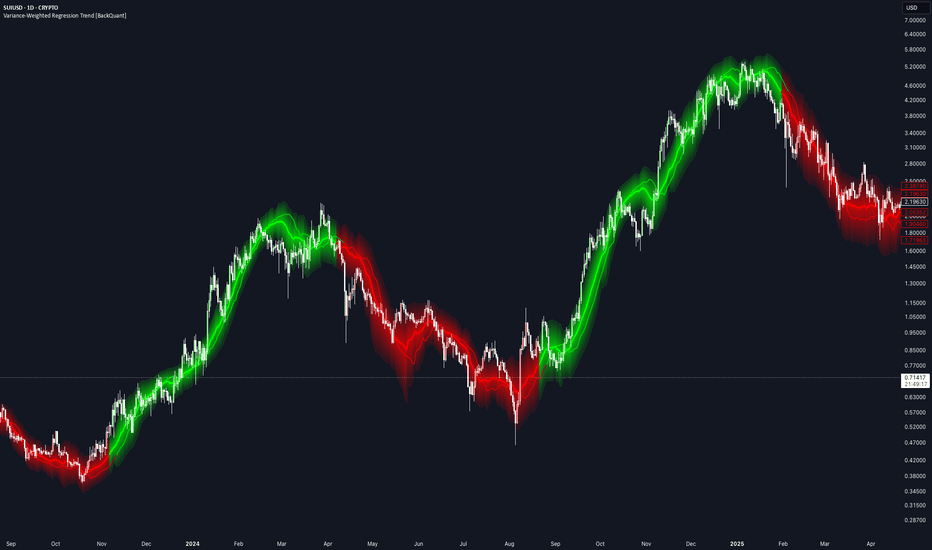
MovTrend Pullback SystemWhat it is: A trend-following 5 minute indicator built around a linear regression trend line ("MovTrend") with ATR-based volatility bands. It generates four distinct signal types, each answering a different question about price action relative to the trend.
Core components
MovTrend Line (MT) — A linear regression line (ta.linreg) plotted over price, colored by direction: green when sloping up, red when sloping down, gray when flat. This is the trend backbone everything else references.
Slope — The MT line's rate of change over a lookback window, plotted as a histogram in the lower pane. Crossing above/below configurable thresholds marks a "confirmed" up or down trend (green/red bars); values between thresholds are a gray "no-trade zone" where the trend isn't strong enough to trust.
ATR Bands — Upper/lower bands plotted around the MT line at a multiple of ATR, representing a "normal" volatility envelope. Price moving outside these bands is considered stretched/overextended relative to the trend.
The four signals
🟢 Buy Dot / 🔴 Sell Dot (Pullback Touch)
Fires when price dips down and touches the MT line during a confirmed uptrend (buy), or pokes up and touches it during a downtrend (sell), then closes back in the trend's favor. This is the core "buy the dip / sell the rip" signal — a shallow pullback to the trend line that holds.
🟡 Stretch Dot (Mean-Reversion Warning)
Fires when price closes outside the ATR bands — i.e., stretched further from the trend line than normal volatility would suggest. Dot size scales with how extreme the stretch is (tiny = mild, small = moderate, orange/normal = extreme), giving you an at-a-glance read on how overextended price is. This isn't a reversal signal on its own — it's a caution flag that price may be due to snap back toward the MT line. It's filtered by:
Volatility regime — suppressed during low-volatility chop, since a "stretch" in dead conditions is less meaningful
FVG confluence — checks if price is near a fair value gap, adding context to the stretch
Volume — requires above-average volume to confirm real participation, not just a thin drift
Slope deceleration — confirms the trend itself is actually losing momentum, not just that price poked outside the band
🔷 Trend Continuation Diamond (cyan up / magenta down)
Fires on a high-volume push with the trend, away from the MT line — meant to catch strong continuation moves the pullback-touch signal misses (since it only fires on touches, not on strength). It's built specifically to avoid firing at exhaustion tops/bottoms by requiring:
Volume that is not the largest in the recent lookback window (avoids climactic blow-off bars)
Slope that's still accelerating, not flattening
A cooldown between diamonds so one strong leg doesn't spam multiple signals
Filters that apply across signals
Session filter — dims the chart and can gate signals outside your configured trading hours, since overnight/thin-liquidity behavior isn't comparable to regular session action
MTF confirmation — optionally requires a higher timeframe's slope to agree before a buy/sell touch fires, filtering out signals that look right locally but fight the bigger picture
Signal conflict resolution — a Trend Continuation diamond won't fire on the same bar as a Buy/Sell touch, avoiding mixed signals
Performance tracking table
How to read it together
The intended workflow: use the MT line + slope histogram to establish trend context, take Buy/Sell touches as primary pullback entries in the direction of that trend, treat Stretch dots as a caution/take-profit signal rather than a new entry, and use Continuation diamonds as confirmation that a trend still has legs when you're already in a position or considering adding. 指标

Polynomial & Logarithmic Regression Channels [OnlyFibonacci]Polynomial & Logarithmic Regression Channels is an overlay indicator that fits a 2nd-degree polynomial regression curve to recent price action and builds dynamic standard deviation channels around that curve. Unlike a straight linear regression line or a simple moving average, the polynomial model captures curved trends — acceleration, deceleration, and rounded turning phases — while deviation bands quantify how far price has stretched from the fitted trend.
What Makes This Indicator Different Matrix-based polynomial regression — Coefficients are solved via least-squares using Pine Script v6 matrix operations (matrix.new, matrix.transpose, matrix.mult, matrix.inv), not a basic ta.linreg() call. Logarithmic price scale toggle — Switch between standard and log-price regression. Log mode is well suited for long-horizon assets where percentage growth matters more than absolute price moves. Residual volatility channels — Inner (±1σ) and outer (±2σ) bands are built from the standard deviation of price residuals relative to the fitted curve, not from raw price volatility alone. Live dashboard — Model type, channel position (%), residual volatility, and trend status (Overbought / Oversold / Neutral) are displayed in an upper-right table. Built-in alerts — Outer channel breaches and polynomial slope direction changes.
How It Works On each bar, the script collects the last N closing prices (default: 200) and fits the equation y = a + bx + cx² using matrix least-squares: β = (X'X)⁻¹X'Y. The regression line value at the current bar becomes the central trend curve. Residuals (actual price minus fitted value) across the lookback window are used to compute a sample standard deviation. Upper and lower channels are then plotted at user-defined σ multipliers. When Use Logarithmic Price Scale is enabled, prices are transformed with math.log() before regression and mapped back to the chart with math.exp() for display. The central line color reflects the instantaneous slope of the polynomial at the current bar: bright green when sloping up, bright red when sloping down.
Key Settings Lookback Period (default 200) — Number of bars used to fit the polynomial. Higher values produce a smoother, slower-reacting curve; lower values track price more closely. Use Logarithmic Price Scale — Enable for long-term trending markets (equities, crypto, indices). Keep off for short-term or range-bound analysis. Inner / Outer Multipliers (default ±1.0 / ±2.0) — Control channel width. Wider multipliers reduce false overbought/oversold signals; tighter multipliers increase sensitivity. Visual Style — Trend colors, band colors, fill transparency, and line widths. Dashboard — Toggle the info table and adjust text size.
How to Read the Chart Polynomial Regression line — The dynamic trend curve. Color shows current slope direction. Inner bands (±1σ) — Normal fluctuation zone around the trend. Pullbacks into inner bands within a trending market may offer continuation setups. Outer bands (±2σ) — Statistical stretch zone. Price beyond outer bands signals extended deviation from the fitted trend. Channel fills — Soft shaded areas between bands help visualize channel structure without cluttering the chart.
Dashboard Metrics Model Type — "Polynomial" (standard scale) or "Log-Poly" (logarithmic scale). Channel Position (%) — Where price sits within the outer channel (0% = outer lower, 100% = outer upper). Values above 80% or below 20% are highlighted. Residual Volatility — Dispersion of price around the fitted curve, shown as a percentage. Trend Status — Overbought (above outer upper), Oversold (below outer lower), or Neutral (inside outer bands).
How to Use — Practical Interpretation Trend identification: Trade in the direction of the regression line color. A green (upward-sloping) curve supports bullish bias; red supports bearish bias. Pullback entries: In a strong trend, price pulling back toward the regression line or inner band while slope remains favorable can indicate a potential continuation zone — always confirm with your own structure or confluence. Mean reversion / exhaustion: When price pushes beyond the outer bands and dashboard shows Overbought or Oversold, the move may be statistically extended relative to the fitted curve. This does not guarantee reversal; it flags stretched conditions. Log vs. standard mode: Use log mode on higher timeframes and growth assets. Use standard mode on lower timeframes or when absolute price deviation is more relevant. Lookback tuning: Match lookback to your analysis horizon — e.g. 100–150 for swing trading, 200+ for position trend context.
Built-in Alerts Overbought — price above outer upper channel Oversold — price below outer lower channel Trend slope turned bullish — polynomial derivative crossed above zero Trend slope turned bearish — polynomial derivative crossed below zero
Recommended Setup Apply to a clean chart with no other overlapping indicators for clearest visualization. Start with default settings (200 lookback, ±1σ / ±2σ bands). Test on your preferred timeframe and symbol before relying on signals. Combine with support/resistance, volume, or higher-timeframe trend for confluence — this tool provides statistical context, not standalone trade signals.
This indicator is a quantitative analysis tool for educational and informational purposes only. It does not constitute financial advice, investment recommendation, or a guarantee of future performance. Past behavior of regression channels does not predict future results. Always manage risk and conduct your own due diligence before making trading decisions.
Credits Developed by OnlyFibonacci . Licensed under Mozilla Public License 2.0. 指标

Regression Channel AutoRegression Channel Auto is a visual trend-structure tool based on least-squares linear regression.
The script draws a regression channel on the chart using either a fixed lookback length or an automatically selected best-fit length. In Auto mode, the script evaluates the available lookback lengths between the user-defined minimum and maximum settings, then selects the window with the highest absolute Pearson correlation. This helps identify the recent price segment that is most closely aligned with a straight-line regression structure.
What the script shows
- A center regression line
- Inner regression bands
- Outer regression bands
- Optional channel fill
- Direction-based coloring for rising, falling, or flat channel slopes
- Optional visual extension to the right
- Optional outside-channel break markers
- Optional alerts for closes outside the outer channel
How it works
The script calculates a least-squares regression line over the selected lookback window. It then measures the residual deviation around that regression line and plots inner and outer bands at user-defined deviation distances.
The channel color changes according to the slope of the regression line:
- Rising channel: positive slope above the flat threshold
- Falling channel: negative slope below the flat threshold
- Flat channel: slope inside the selected flat threshold
Auto Length mode
In Auto mode, the script scans the lookback range selected by the user and chooses the length with the strongest absolute Pearson correlation. This means the selected channel is the one whose recent price structure is most linear within the evaluated range.
A high correlation value describes how closely price followed a linear path during the selected window. It does not predict future price movement.
Fixed Length mode
Fixed mode uses one user-defined lookback length. This is useful when the user wants a stable channel length instead of an automatically changing one.
Main settings
Channel:
- Length mode
- Fixed length
- Auto minimum length
- Auto maximum length
- Source
- Flat threshold
Bands:
- Inner band deviation
- Outer band deviation
- Show inner bands
- Show channel fill
Display:
- Extend channel right
- Show info label
- Show current outer break marker
Lines:
- Center line width
- Inner band width
- Outer band width
- Center line style
- Inner band style
- Outer band style
Colors:
- Rising channel color
- Falling channel color
- Flat channel color
- Inner band transparency
- Channel fill transparency
Alerts
The script includes optional alert conditions for:
- Close above the upper outer regression channel
- Close below the lower outer regression channel
These alerts describe price moving outside the selected regression channel. They are not buy or sell signals.
How to use
Use this indicator to review whether price is moving inside a structured linear channel, near the upper or lower side of the channel, or outside the outer deviation bands.
The tool can be useful for visual trend review, mean-deviation context, and identifying when price has moved outside its recent regression structure.
Important note on refitting
This script is recalculated as new bars develop. In Auto mode, the selected lookback length can also change when new price data changes which window has the highest absolute Pearson correlation.
For this reason, the channel should be understood as a dynamic descriptive tool. It is not a fixed historical signal and it should not be interpreted as a prediction model.
Limitations
- The channel is based on recent price structure only.
- A high Pearson correlation measures linearity, not future performance.
- A close outside the channel does not automatically mean continuation or reversal.
- Outer-band contact is not a standalone trading signal.
- The optional right extension is a visual reference only and is not a forecast.
This indicator is intended for chart analysis, educational use, and visual review of regression-channel structure. 指标

AUTO TRENDLINE PROauto trendline pro
auto trendline pro is an automatic trendline indicator designed to display multiple degrees of market structure at the same time: live trendlines, confirmed trendlines, and higher timeframe trendlines.
the purpose of the tool is to help traders identify dynamic support and resistance lines, projected levels, confirmed breaks, and higher timeframe structure directly on the chart.
the indicator uses pivot points, wick or body anchors, atr-based validation, touch detection, duplicate filtering, forward projection, optional channels, and a dashboard for fast market reading.
it can be used for scalping, intraday trading, swing trading, and macro analysis depending on the selected settings.
---
inputs guide
degrees
live degree
enables live trendlines. this mode reacts faster to recent price action, but it can repaint because the pivots are still developing. it is useful for short-term market reading and early structure detection.
confirmed degree
enables confirmed trendlines. this mode is more stable because it uses confirmed pivots. it is recommended for cleaner analysis and more reliable structural levels.
htf degree
enables higher timeframe trendlines. this mode brings larger market structure into the current chart and helps identify major dynamic support and resistance levels.
anchor source
selects how the trendline anchors are calculated.
wick uses candle highs and lows.
body uses candle open and close extremes.
wick is more aggressive and reacts to full price extremes. body is cleaner and can reduce noise.
---
pivot strength
live pivot l/r
controls the strength of live pivots. a lower value creates more reactive trendlines. a higher value creates fewer but cleaner lines.
confirmed pivot l/r
controls the strength of confirmed pivots. a higher value makes the confirmed trendlines more selective and more structural.
htf pivot l/r
controls the pivot strength used on the higher timeframe. higher values create more macro-level lines.
---
htf source
htf timeframe
selects the higher timeframe used for htf trendlines. examples: 4h, 1d, 1w. higher timeframes provide stronger macro structure.
htf ath/atl window
defines the lookback window used to detect higher timeframe highs and lows. a larger value allows the indicator to anchor lines to more important historical extremes.
anchor htf line at ath / atl
allows htf lines to be anchored from the highest high or lowest low inside the selected htf window. this is useful for long-term trendlines and cycle analysis.
htf compute in log space
calculates htf trendlines using logarithmic logic. this is useful for assets with large percentage moves, such as crypto, because it gives a more balanced macro structure.
---
structure and validation
lines per side chart degrees
defines how many chart-degree lines are displayed per side. increasing this value shows more trendlines but can make the chart busier.
lines per side htf
defines how many higher timeframe lines are displayed per side. a lower value keeps the chart cleaner. a higher value gives more macro context.
new-anchor candidates
defines how many recent pivots are tested as possible new anchors. higher values test more combinations.
older-anchor window
defines how many older pivots can be used with a recent pivot to create a valid trendline.
min bars between anchors
defines the minimum distance between two trendline anchors. a low value creates shorter lines. a higher value creates more meaningful structural lines.
allowed pierces
defines how many times price is allowed to pierce a line during validation. zero means strict validation.
pierce tolerance atr
defines the atr-based tolerance used when checking if price has pierced a line. a lower value is stricter. a higher value allows more flexibility.
touch tolerance atr
defines the atr-based tolerance used to count touches on a trendline. a higher value detects more touches. a lower value keeps only precise touches.
dedupe distance atr
filters trendlines that are too close to each other. a higher value removes more duplicate lines.
max validation span
defines the maximum number of bars used when validating a trendline. this prevents the indicator from validating lines across an excessive historical distance.
---
channels, break and extension
show channels
enables channels around the dominant trendline. channels help visualize the reaction area around a trendline instead of focusing only on a single line.
break = n consecutive closes beyond
defines how many consecutive candle closes are required to confirm a break. a value of 1 is faster. a value of 2 or more is stricter.
forward projection bars
defines how far the trendlines are projected into the future.
infinite extension
extends the lines continuously to the right. this is useful when using trendlines as ongoing dynamic support and resistance.
---
display
price projection label
shows the projected price at the end of a trendline. this helps identify the current reaction level quickly.
show trendline labels
enables or disables labels on trendlines. keeping this off gives a cleaner chart.
strength rating
shows a visual strength rating based on the number of valid touches. more touches generally mean a more important line.
show dashboard
enables the dashboard. the dashboard summarizes confirmed support, confirmed resistance, htf support, htf resistance, htf extremes, and validation status.
dashboard position
selects the position of the dashboard on the chart.
---
aesthetics
support
sets the color of support trendlines.
resistance
sets the color of resistance trendlines.
htf glow / accent
sets the accent color used for higher timeframe emphasis.
broken
sets the color used when a trendline is broken.
atr length
defines the atr length used for tolerances, validation, touch detection, break detection, and duplicate filtering.
---
how to use the indicator
start by using confirmed degree and htf degree. these two modes give the cleanest structure.
live degree is useful for faster market reading, but beginners should understand that live pivots can repaint while they are forming.
support lines are usually below price and can act as dynamic reaction zones.
resistance lines are usually above price and can act as dynamic rejection zones.
when price approaches a confirmed or htf trendline, watch how it reacts. price can reject the line, break through it, or compress near it before a stronger move.
a break is cleaner when price closes beyond the line. this is why the break confirmation input is important.
---
beginner tutorial
1. choose your trading timeframe, such as 15m, 1h, 4h, or 1d.
2. enable confirmed degree to display stable trendlines.
3. enable htf degree to display higher timeframe structure.
4. keep live degree enabled only if you want more reactive lines.
5. wait for price to approach a support or resistance trendline.
6. observe the candle reaction near the line.
7. a rejection can indicate that the line is still respected.
8. a confirmed close beyond the line can indicate a structural break.
9. use the dashboard to monitor the main confirmed and htf levels.
10. never use a trendline alone as a full trade signal. combine it with market structure, volume, candles, liquidity, and risk management.
---
simple beginner setup
live degree: off
confirmed degree: on
htf degree: on
anchor source: wick
confirmed pivot l/r: 10
htf pivot l/r: 8
allowed pierces: 0
break = n consecutive closes beyond: 2
show channels: on
show trendline labels: off
show dashboard: on
this setup keeps the chart clean and focuses on confirmed structure.
---
scalping setup
live degree: on
confirmed degree: on
htf degree: on
live pivot l/r: 3 to 5
confirmed pivot l/r: 8 to 12
break = n consecutive closes beyond: 1 to 2
forward projection bars: 10 to 30
show trendline labels: off
this setup gives faster signals and more reactive structure, but it should be used with more caution.
---
swing trading setup
live degree: off
confirmed degree: on
htf degree: on
confirmed pivot l/r: 10 to 20
htf pivot l/r: 8 to 15
htf timeframe: 1d or 1w
htf compute in log space: on for crypto
break = n consecutive closes beyond: 2 or 3
infinite extension: on
this setup focuses on larger trendlines and reduces short-term noise.
---
dashboard guide
conf resist
shows the main confirmed resistance trendline level.
conf support
shows the main confirmed support trendline level.
htf resist
shows the main higher timeframe resistance trendline level.
htf support
shows the main higher timeframe support trendline level.
htf ath / atl
shows the higher timeframe extreme levels used for macro context.
validation
shows that the lines are built using structure and validation logic.
---
important notes
a trendline is not an automatic buy or sell signal.
a trendline is a decision zone.
the more clean touches a line has, the more important it becomes.
a close beyond a line is usually more important than a wick through the line.
higher timeframe lines should always be respected because they represent larger market structure.
this tool is designed to organize chart structure, but risk management remains essential.
指标

Volumetric Regression Heatmap [LuxAlgo]The Volumetric Regression Heatmap indicator is a sophisticated market analysis tool that combines dynamic linear regression with volume profile density to visualize fair value and liquidity zones. By projecting volume-weighted heatmaps within a trend-following channel, it allows traders to identify where the bulk of trading activity has occurred relative to the current price trajectory.
🔶 USAGE
The indicator provides a multi-layered view of market structure. The central heatmap shows the "hottest" areas of volume concentration, acting as a magnet for price, while the outer bands represent statistical extremes.
🔹 Mean Reversion Signals
The script includes a built-in signal system designed for sideways or "flat" markets. When the indicator detects a "Contraction" state (determined by the ratio of channel height to standard deviation), it plots small circles at the +2/-2 standard deviation levels.
Green Circles: Potential long opportunities when price crosses below the lower signal band during a flat market.
Red Circles: Potential short opportunities when price crosses above the upper signal band during a flat market.
🔹 Future Projections & Profile
The heatmap extends beyond the current bar, providing a "Future Projection" zone. This allows traders to anticipate where support and resistance levels will be in the coming sessions. To the right of the projection, a Bookmap-style volume profile histogram displays the total volume distribution, helping to identify high-volume nodes (HVN) and low-volume nodes (LVN) at a glance.
🔶 DETAILS
🔹 Dynamic Auto-Adjusting Period
Unlike standard regression channels that use a fixed lookback, this tool features an adaptive engine. It calculates the ratio between short-term and long-term volatility (ATR).
In high-volatility environments, the channel period shrinks to become more reactive.
In low-volatility or ranging environments, the period expands to capture a broader structural view.
🔹 Volumetric Delta Histograms
The script calculates the approximate buying and selling volume for every candle within the lookback period. This data is visualized as histograms extending from the outer bands:
Top Band (Green): Displays buying pressure delta.
Bottom Band (Red): Displays selling pressure delta.
This allows traders to see not just where price is, but the intensity of the volume driving it toward the channel extremes.
🔶 SETTINGS
🔹 Core Settings
Source: The price source used for the regression calculation.
Base Period: The anchor length for the regression fit.
Dynamic Auto-Adjusting Period: Enables/disables the volatility-based adaptive lookback.
🔹 Heatmap Settings
Grid Rows Each Side: Determines the vertical resolution of the heatmap bands.
Gradient Smoothing: Applies a smoothing algorithm to the volume distribution for a cleaner visual gradient.
Colors 1-5: Customizable colors ranging from low-volume areas to high-volume "hot" zones.
🔹 Mean Reversion Signals
Signal Band (SD Multiplier): The standard deviation level required to trigger a signal.
Flat Slope Threshold: Controls how "flat" the channel must be to allow signals to appear, preventing counter-trend signals in strong trending markets.
🔹 Delta Histograms
Histogram Height Scale: Adjusts the vertical magnitude of the delta bars.
Histogram Bar Width: Sets the thickness of the individual delta lines.
🔹 Style & Options
Future Projection Length: How many bars to project the heatmap into the future.
Show Volume Profile Histogram: Toggles the right-sided volume distribution boxes.
🔹 Dashboard
Dashboard: Toggles the on-screen analytics panel.
Position/Size: Adjusts the location and scale of the dashboard UI.
指标

指标

指标

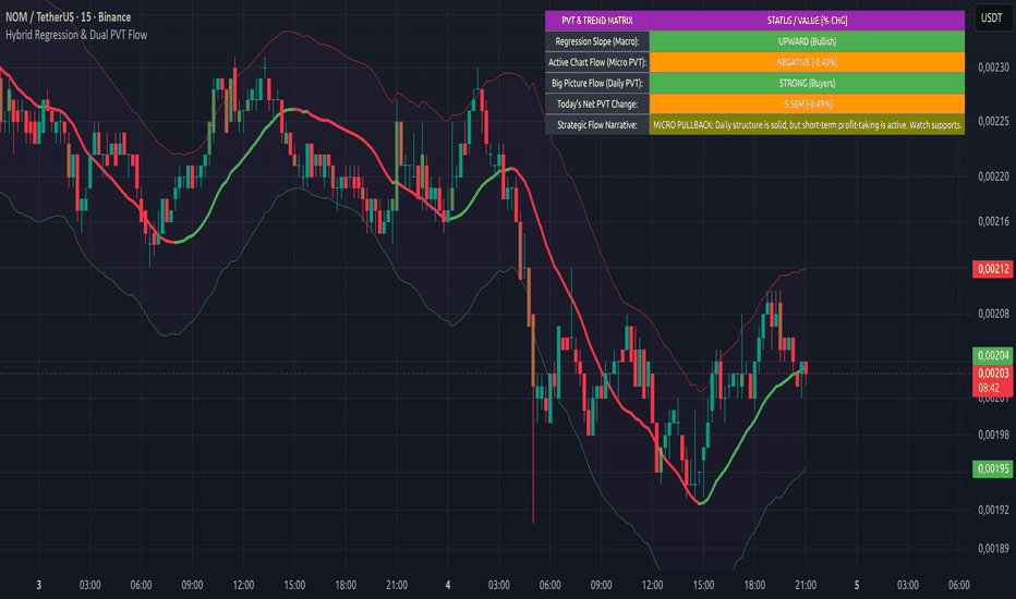
Hybrid Regression & Dual PVT Flow🇺🇸 ENGLISH DESCRIPTION TEXT
Overview
Hybrid Regression & Dual PVT Flow is an institutional-grade hybrid analysis system designed to uncover the footprints of market whales. It bridges the gap between pure price geometry and volume-weighted momentum, preventing retail traders from falling into "bull/bear traps" by exposing hidden institutional accumulation and distribution phases.
Key Technical Pillars:
Linear Regression Core: Computes a noise-filtered baseline representing the true mathematical equilibrium of price. The curve turns green during a bullish slope and red during a bearish slope.
Dynamic Fibonacci Volatility Envelope: Employs an ATR-driven deviation mechanism instead of traditional standard deviations. It projects key institutional overbought (Resistance) and oversold (Support) thresholds based on the 2.618 Fibonacci ratio.
Volume Anomaly Engine: Scans for extreme institutional anomalies where candle volume exceeds 1.5x of its 20-period moving average. These high-activity institutional bars are highlighted in Yellow on your chart.
Dual-Layer Multi-Timeframe PVT Dashboard:
Micro PVT Status: Tracks real-time smart money participation directly on your active trading timeframe (e.g., 5m, 15m, 1h).
Macro PVT Status: Permanently anchors a Daily (1D) Price Volume Trend core against its 10-period EMA, providing an unshakeable perspective of the "Big Picture" regardless of your active asset chart.
How to Read the Intelligence Dashboard:
BULLISH / BEARISH CONVERGENCE: Absolute alignment between the macro trend line and multi-timeframe capital flows. Indicates high-probability trend continuation.
HIDDEN BEARISH DIVERGENCE (Distribution Trap): Price regression slope is upward, but both macro and micro PVT metrics are flashing negative. Highly indicative of institutional selling into retail FOMO.
STRONG ACCUMULATION DIVERGENCE (Whale Accumulation): Price regression slope is sliding downward, but dual-layer PVT inflows are accelerating heavily. Signals structural retail liquidation being absorbed by institutional market makers right before a major reversal.
🇹🇷 TÜRKÇE AÇIKLAMA METNİ
Özet Giriş
Hybrid Regression & Dual PVT Flow, piyasada sıklıkla karşılaşılan "fiyat yükselirken kurumsal oyuncuların arka kapıdan mal çıkması" (dağıtım) veya "fiyat düşerken balinaların dipten gizlice mal toplaması" (akümülasyon) durumlarını yakalamak için tasarlanmış hibrit bir takip sistemidir. Matematiksel gücünü Doğrusal Regresyon Eğrisi ve Çift Katmanlı Price Volume Trend (PVT) momentum motorunun sentezinden alır.
Ana Özellikler:
Doğrusal Regresyon Hattı (Linear Regression Trend): Piyasanın ana dengesini ve makro yönünü gürültüden arındırılmış bir eğri olarak sunar. Eğim yukarıysa yeşil (Boğa), aşağıysa kırmızı (Ayı) olarak grafiğe işlenir.
Dinamik Fibonacci Volatilite Bantları: Klasik Bollinger bantları yerine, ATR (Average True Range) tabanlı dinamik volatilite sınırları kullanır. Üst kırılımlar kurumsal aşırı alım/direnç, alt bantlar ise kurumsal güvenli alım/destek bölgelerini işaret eder.
Hacim Anomalisi Mum Boyama: Son 20 mumun ortalama hacmini %150 aşan ani balina aktivitelerinde, mumlar otomatik olarak Sarı renge boyanarak dikkat çeker.
Çift Katmanlı PVT ve Trend Matris Paneli: * Mikro PVT: Bulunduğunuz anlık aktif grafik zaman dilimindeki (5dk, 15dk, 1sa vb.) para akışı yönünü ölçer.
Makro PVT: Grafiğiniz ne olursa olsun, arka planda Günlük (1D) kurumsal para akışının 10 günlük ortalamasını denetler.
Panel Strateji Notları Nasıl Okunur?
TAM UYUM (BOĞA / AYI): Trend yönü ile tüm vadelerdeki para akışları aynı yöndedir. Güvenli katılım bölgesidir.
GİZLİ AYI UYUMSUZLUĞU (Dağıtım Tuzağı): Regresyon eğrisi yukarı bakarken, hem günlük hem anlık para akışları negatif yönlüdür. Balinaların küçük yatırımcıya mal devrettiği tepe tuzaklarını gösterir.
GİZLİ BOĞA UYUMSUZLUĞU (Mal Toplama): Grafik aşağı akarken, hem günlük hem anlık PVT'nin güçlü yönlü yukarı gitmesidir. Balinaların dipten toplama yaptığını ve sert bir yükselişin yakın olduğunu gösterir. 指标
Sloped LinReg Volume Profile [MarkitTick]💡 This indicator introduces a highly dynamic approach to volume and price analysis by merging standard volume principles with vector-based linear regression. Rather than plotting volume distributions on a static horizontal plane, this tool maps volume nodes parallel to the prevailing mathematical trend. By constructing a localized volume profile that follows the trajectory of price action, it captures momentum-adjusted value areas, providing an advanced lens for interpreting market geometry, support/resistance, and volume anomalies. It is strictly engineered for standard candlestick charts, specifically excluding non-standard formats to ensure pristine volume and price data integrity.
● ✨ Originality and Utility
Standard volume profiles aggregate historical volume at fixed price levels, which often creates fragmented or obsolete value nodes when a market is actively trending. This indicator resolves that structural limitation by angling the volume bins to match the slope of a linear regression channel.
It identifies where volume is concentrated relative to the trend's axis, not just the absolute price.
It reveals volume-weighted momentum, highlighting whether buying or selling pressure is accelerating in the direction of the regression slope.
The tool includes an integrated, dark-mode optimized analytics dashboard that processes quantitative metrics natively on the chart without requiring secondary oscillators.
● 🔬 Methodology and Concepts
The foundational logic relies on computing a rolling linear regression to establish a baseline trajectory over a specified period. The methodology relies on Pine Script's time-series event loop, evaluating arrays of data dynamically as new bars form.
Vector-Based Binning: Instead of horizontal rows, the profile utilizes a dynamic upper and lower deviation band. The mathematical distance between these bands is partitioned into a user-defined number of rows.
Volume Distribution: As the script loops through the historical lookback window, it evaluates the volume of each bar. The volume is divided proportionally across the sloped bins that intersect the bar's high-low range.
Directional Volume (Delta): Each bin further categorizes volume into "Buy" or "Sell" categories based on whether the bar's closing price was greater than or equal to its opening price.
Value Area Calculation: The Point of Control (POC) identifies the sloped bin with the highest total volume. The Value Area High (VAH) and Value Area Low (VAL) expand outward from the POC until they encapsulate a specific percentage of the total allocated volume, dynamically updating as price action develops.
● 🎨 Visual Guide
Every visual element is rendered utilizing Pine Script's advanced drawing arrays and is fully user-configurable to support dark-mode analytical environments.
• The Sloped Profile
Volume Bars: Rendered as polygons extending inward from the right side of the channel. The length of each polygon represents the relative volume allocated to that specific standard deviation bin.
Color Coding: Bullish volume defaults to a translucent teal, while bearish volume displays as a translucent red. Bins experiencing extraordinary volume influxes override with a bright, high-visibility color to highlight anomalous market participation.
• Channel and Level Lines
Regression Bounds: Solid or semi-transparent lines mapping the start and end of the regression channel, defining the upper and lower standard deviation extremes.
POC Line: A thick, solid yellow line plotting the Point of Control across the length of the channel.
Value Area Lines: Dashed blue lines tracking the VAH and VAL. The area between these lines is shaded with a deep blue fill to instantly highlight the trend's core acceptance zone.
Delta POC: A dashed fuchsia line identifying the bin with the most extreme difference between buying and selling volume.
• Analytics Dashboard
Located in the top right, this table provides real-time quantitative readouts formatted to precise tick values.
LinReg Slope: Indicates the mathematical direction of the trend (Bullish/Bearish).
Price Regime: Identifies if the current close is inside the channel or breaking the upper/lower bounds.
Volume POC & Delta POC: Displays the exact price equivalents of the sloped control lines at the current bar index.
Buy Vol Bias: A visual progress bar detailing the ratio of bullish to bearish volume within the regression window.
Vol Compression: Evaluates the density of the value area. A highly concentrated value area yields a higher compression score.
● 📖 How to Use
The indicator serves as a complete environmental map for trending markets.
Trend Qualification: Utilize the slope of the regression channel to establish the primary directional bias. Trades should ideally align with the slope.
Value Area Rejections: The VAH and VAL lines function as dynamic support and resistance. A price action rejection at the VAH within a downward-sloping channel offers a high-probability continuation setup.
POC Magnetism: Price will naturally gravitate toward the sloped POC. Deviations far outside the Value Area typically mean-revert to the POC unless accompanied by a severe volume imbalance.
Interpreting Delta: Compare the traditional POC to the Delta POC. If the Delta POC rests significantly higher or lower than the overall Volume POC, it indicates an aggressive concentration of directional absorption (trapped buyers or sellers).
Repainting Warning: Because this indicator calculates a dynamic linear regression over a moving lookback window, the visual placement of the channel and profile will continually recalculate and shift on the real-time bar until the bar closes. This is standard behavior for dynamic geometric overlays, but users should wait for bar confirmation before executing trades based on channel interactions.
● ⚙️ Inputs and Settings
• Linear Regression Settings
Channel Length: Defines the historical lookback window (default is 100). Higher values create smoother, macro-trend profiles.
Source: The price data used for the regression calculation (Open, High, Low, Close, HL2, HLC3, OHLC4).
Upper/Lower Deviation: Toggles the outer bounds of the channel and sets the standard deviation multipliers.
• Sloped Volume Profile Settings
Number of Rows: The granularity of the profile. More rows create thinner, more precise volume nodes.
Profile Width %: Determines how far the volume polygons stretch across the screen relative to the channel length.
Value Area %: The percentage of total volume to include within the VAH and VAL bounds (default 70%).
• Advanced Quant Analytics
Highlight Footprints: Visually isolates volume bins that exceed two standard deviations above the mean bin volume.
Calculate Anchored VWAP: Toggles the inclusion of an Anchored VWAP (anchored to the start of the regression window) within the dashboard matrix.
⚠️ Disclaimer
All provided scripts and indicators are strictly for educational exploration and must not be interpreted as financial advice or a recommendation to execute trades. I expressly disclaim all liability for any financial losses or damages that may result, directly or indirectly, from the reliance on or application of these tools. Market participation carries inherent risk where past performance never guarantees future returns, leaving all investment decisions and due diligence solely at your own discretion. 指标

指标

Z-Score Probability Pro KAMA
Z-Score Probability Pro KAMA, v1.0 by Erika Barker
Hey guys, this is the successor to my original Z-Score Probability HMA Indicator, which you can still use if you prefer that one.
This is version 1.0 of the new rebuild, and it is a pretty big upgrade. The goal was to keep the statistical foundation that made the original useful, but make it more adaptive, cleaner, and better at understanding different market conditions.
What is new
1. Timeframe auto-adaptation
No more constantly re-tuning the indicator when you switch charts.
The lookback now automatically adjusts based on the chart timeframe, using a calendar-style window, defaulting to about 5 trading days. The dashboard also shows the effective lookback being used, so you always know what the script is calculating from.
It works from 1 minute charts all the way up to weekly charts.
2. Better smoothing logic
The original HMA was doing a lot of work at once. In this version, the baseline and the Z-score smoothing are separated so each one can do its own job better.
By default:
* Baseline: KAMA, great for adapting to noisy markets
* Z-score smoothing: ALMA, smoother and cleaner on the oscillator
HMA is still available if you prefer the original feel.
3. Modified Z-Score option
There is now an optional Modified Z-Score mode using MAD, median absolute deviation.
This is useful for markets with big outliers, fat tails, sudden spikes, crypto moves, small caps, and anything that tends to behave a little wild.
When this mode is turned on, the threshold bands automatically adjust.
4. Regime filter using Hurst logic (been needing out on this a lot lately on personal stuff)
This version attempts to classify the market as:
* Trending
* Mean-reverting
* Random
That matters because an extreme Z-score does not always mean the same thing.
In a mean-reverting market, an extreme Z-score can suggest exhaustion.
In a trending market, that same extreme can sometimes mean continuation or breakout strength.
This was one of the biggest things I wanted to improve from the original.
5. Divergence engine
The indicator now includes both regular and hidden divergence.
It can detect:
* Regular bullish divergence
* Regular bearish divergence
* Hidden bullish divergence
* Hidden bearish divergence
Divergences are confirmed using pivots, so they are non-repainting, but they will appear a few bars after the actual pivot. That is the tradeoff for confirmation.
6. Higher-timeframe confirmation
The script can pull Z-score confirmation from a higher timeframe.
You can use the automatic HTF mode or set it manually. HTF values only update after the higher-timeframe candle closes, so this is designed to avoid repainting.
7. Strong Buy and Strong Sell signals
Signals are based on a confluence score instead of just one condition.
The score looks at things like:
* Z-score reversal
* Divergence
* Baseline slope
* Market regime
* Higher-timeframe agreement
* Volume confirmation, when volume is available
You can choose the conviction level:
* Low
* Medium
* High
Medium is the default and should give fewer, cleaner signals.
8. Live dashboard
The dashboard shows:
* Detected timeframe
* Effective lookback
* Current Z-score
* Market regime
* Hurst value
* Higher-timeframe status
* Bull and bear scores
* Conviction threshold
* Last signal
You can move it to any corner of the chart.
9. More stable defaults
The defaults were chosen to be centered in stable performance zones, not over-optimized for one market.
Basically, I did not want this to be something that only looks good on one ticker, one timeframe, during one perfect backtest window.
10. Built in Pine v6
This version uses Pine v6 features, including dynamic higher-timeframe requests and confirmed-bar alert logic.
Repaint disclosure
This indicator is designed to avoid repainting, but there are a few things to know:
* Divergence and Strong Buy/Sell labels appear after pivot confirmation, default is 3 bars later
* Higher-timeframe confirmation only updates after the higher-timeframe candle closes
* Alerts fire on confirmed bars, not intrabar ticks
So, signals are delayed slightly by design, but that is what makes them confirmed.
How to use it
Beginner
Leave everything on default.
Watch the dashboard and look for:
* Strong Buy
* Strong Sell
Medium conviction is probably the best starting point.
Intermediate
Try the Modified Z-Score mode on crypto, small caps, or anything with sharp moves and big outliers.
Turn on Hidden Divergence if you like trading trend continuation setups.
Advanced
You can tune the component weights to match your own strategy.
The indicator is flexible, so you can make it more reversal-focused, more trend-following, or more confirmation-heavy depending on your trading style. 指标

Linear Regression Scanner (KenshinC)Linear Regression Scanner (KenshinC) + Slope Visual is a powerful real-time multi-symbol dashboard combined with advanced Linear Regression visualization. It analyzes up to 12 major cryptocurrency pairs simultaneously, displaying trend direction, price position relative to the regression midline, RSI(14), and precise slope values in a clean table. Additionally, it plots the Linear Regression Curve and dynamic slope direction arrows directly on the current chart for deeper visual insight.
🔍 WHAT MAKES IT ORIGINAL
1. True Multi-Symbol Linear Regression Engine — Simultaneously calculates full Linear Regression Channels (intercept, endpoint, deviation, and slope) for 12 symbols using request.security().
2. Dual Linear Regression System — Uses two independent regression calculations: one for the scanner table (default 100 bars) and one for on-chart visualization (default 150 bars) with slope arrows.
3. Slope-Based Trend & Momentum Arrows — Detects trend direction from regression slope and displays intuitive teal/orange arrows showing slope strength on every bar.
4. Price vs Regression Midline Positioning — Real-time comparison of price against the dynamic regression center line.
5. Professional All-in-One Dashboard — Clean, color-coded table with Trend, Price Position, RSI, and Slope — all updated on bar close.
6. Highly Customizable — Independent settings for scanner channel and on-chart regression curve.
⚙️ HOW IT WORKS
The scanner uses a custom get_channel() function to compute the best-fit Linear Regression line as follows:
mid = math.sum(src, len) / len
slope = ta.linreg(src, len, 0) - ta.linreg(src, len, 1)
intercept = mid - slope * math.floor(len / 2) + (1 - len % 2) / 2 * slope
This produces:
- The midline (average of the source over the chosen Channel Length)
- The true slope of the regression line (rate of change)
- Intercept and projected endpoint for accurate current-bar positioning
- Standard deviation around the line (ready for future deviation bands)
Trend is determined directly from the slope: positive slope = Bullish, negative slope = Bearish.
Price vs Middle compares the current price to the regression line value at the current bar.
For the on-chart visualization (inspired by emiliolb):
lrc = ta.linreg(close, lrc_len, 0)
lrprev = ta.linreg(close , lrc_len, 0)
slope_current = (lrc - lrprev)
This plots a smooth red Linear Regression Curve (default 150 bars) and displays slope direction with arrows: Teal ↑ for positive/strengthening slope (bullish momentum) and Orange ↓ for negative/strengthening slope (bearish momentum).
RSI(14) is calculated independently for each symbol to show overbought (>70) and oversold (<30) conditions.
The entire dashboard refreshes on every bar close using efficient array looping.
📖 HOW TO USE
Reading the Dashboard Table (Top Right):
- Symbol: Ticker name (e.g., BTCUSDT)
- Trend: Green = Bullish (positive slope), Red = Bearish (negative slope)
- Price VS Middle: Green = Price above regression midline (bullish positioning), Red = Below midline (bearish positioning)
- RSI: Lime Green (<30) = Oversold, Yellow (30–70) = Neutral, Red (>70) = Overbought
- Slope: Precise numerical value — the higher the positive number, the stronger the uptrend; the lower the negative number, the stronger the downtrend.
Reading On-Chart Visuals:
- Red Curve: Linear Regression Curve (default 150 bars) — serves as a dynamic trend baseline.
- Teal Arrows ↑: Positive and strengthening slope → bullish momentum.
- Orange Arrows ↓: Negative and strengthening slope → bearish momentum.
Suggested Trading Workflow:
1. Scan the table for Bullish symbols showing “Bullish” + “Above” + strong positive Slope.
2. Confirm RSI is not extremely overbought (>70).
3. Switch to the symbol and observe the Red LRC Curve together with Slope Arrows for precise timing.
4. Look for strong confluence: Positive slope + price above midline + teal arrows = high-probability trend continuation setup.
5. Best performance on 15m, 1H, and 4H timeframes.
6. Always combine with support/resistance levels, volume, or higher-timeframe analysis.
Best Practices:
- Use longer Channel Length (100+) for smoother, longer-term trend detection.
- Adjust Linear Regression Length (150) to control the smoothness of the on-chart curve and arrows.
- Works excellently on major USDT perpetual pairs.
⚙️ KEY SETTINGS REFERENCE
- Symbols: 12 pre-loaded major Binance USDT pairs (fully customizable)
- Linear Regression Slope Section: Show Curve, Show Arrows, Length (default 150), Color, Width
- Channel Settings: Source (default = low), Channel Length (default 100), RSI Length (default 14)
- Colors: Up Trend and Down Trend colors
🔔 Alerts
No built-in alerts yet. You can easily create manual alerts for slope direction changes, price crossing the regression midline, or RSI extremes.
⚠️ IMPORTANT NOTES
— On-chart Linear Regression Curve and Slope Arrows are calculated and displayed only for the current symbol you are viewing.
— The scanner table analyzes all 12 symbols independently in real time.
— All calculations are performed on bar close to prevent repainting.
— Slope values are not normalized across different assets — only compare them within the same symbol and timeframe.
— Strong slope signals indicate trend strength but do not guarantee future price movement.
— This indicator uses multiple request.security() calls. Avoid overloading the chart with too many other indicators.
— Past performance is not indicative of future results. This tool is for educational and analytical purposes only.
— Not financial advice. Always use proper risk management and trade at your own risk.
---
Made with passion by KenshinC
Happy trading & trend hunting! 🚀 指标
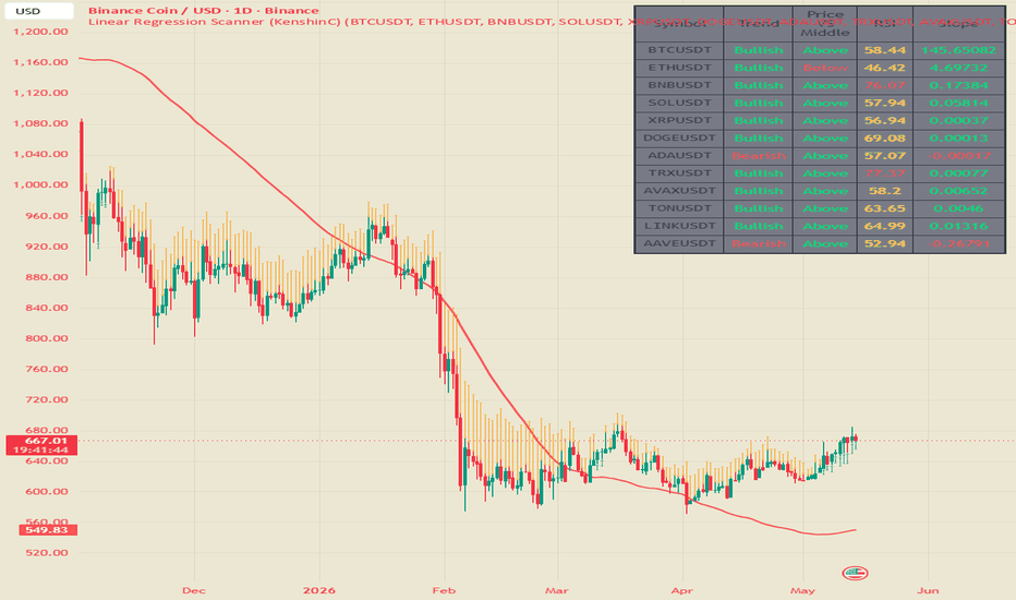
指标

Artemis Regression Bands🟦 Artemis Regression Bands is a kernel-driven volatility envelope indicator built on the KernelLens Nadaraya–Watson regression library (a_jabbaroff/KernelLens/1). A single kernel estimate — selectable from eight classical kernel families — anchors the Fair Value line. Around it, three residual-standard-deviation bands (±1σ, ±2σ, ±3σ) fan outward with either Linear or Exponential spacing, producing a statistically grounded envelope far cleaner than the classical close-stdev approach used by legacy Bollinger-style indicators. A four-gate Romb signal engine overlays buy / sell diamond markers when price pokes through the outermost enabled σ boundary and reverses back inside.
🟦 HOW IT WORKS
Artemis calls the KernelLens library's unified dispatcher once per bar to build the Fair Value line, then queries three additional library exports to derive the band widths, slope direction, and residual σ:
```
fair = kl.estimate (type, src, ℓ, α, period, phase, filter)
sigma = kl.confidenceBand(src, fair, window)
slopeVal = kl.slope (fair, 1)
trendSt = kl.trendState (fair, 1)
dev = baseMult · sigma
upper1 = fair + 1·dev lower1 = fair − 1·dev
upper2 = fair + 2·dev lower2 = fair − 2·dev
upper3 = fair + k3·dev lower3 = fair − k3·dev (k3 = 3 Linear | 4 Exp)
```
The library handles all weighted-sum computation, loop-depth selection, NA-safe iteration, division-by-zero guards, and input validation internally. Artemis contains zero kernel math — every bug fix or optimization in the library automatically propagates to this indicator.
🟦 KERNEL LIBRARY INTEGRATION
Artemis imports the published KernelLens library and uses the following exports:
| Library Export | Used For |
|---|---|
| `kl.estimate()` | Unified dispatcher — routes to the correct kernel based on the user's Kernel Type dropdown. Called once per bar to produce the Fair Value line. |
| `kl.confidenceBand()` | Rolling standard deviation of the (source − Fair Value) residual. Drives the band half-widths on every bar. |
| `kl.slope()` | Discrete first derivative of the Fair Value line. Feeds trend flip alerts. |
| `kl.trendState()` | Ternary classifier (+1 rising / −1 falling / 0 flat) of the Fair Value line. Drives the slope-adaptive color, the kernel trend confluence filter, and the dashboard Trend row. |
Every regression computation — kernel weight evaluation, NA-safe summation, bandwidth-aware loop termination, residual stdev, finite-difference slope — is delegated to the library. The indicator itself only orchestrates the four library calls and layers the visual pipeline on top.
🟦 EIGHT KERNEL FAMILIES
A single Kernel Type dropdown selects any of the eight kernels shipped with the KernelLens library. Each is a different mathematical smoother with its own statistical character:
| Kernel | Formula | Best For |
|---|---|---|
| Rational Quadratic | (1 + d² / (2·α·ℓ²))^(−α) | Multi-scale mixer; α controls stretch. Recommended default. |
| Gaussian / RBF | exp(−d² / (2·ℓ²)) | Canonical smoother; infinitely differentiable. |
| Periodic | exp(−2·sin²(π·d/p) / ℓ²) | Resonates with a known repetition distance p. |
| Locally Periodic | Periodic × Gaussian | Seasonal patterns with slow trend drift. |
| Epanechnikov | (3/4)·(1 − u²), \|u\| ≤ 1 | MSE-optimal; compact support, no tail contamination. |
| Tricube | (70/81)·(1 − \|u\|³)³, \|u\| ≤ 1 | LOWESS standard; near-Gaussian compact profile. |
| Triangular | (1 − \|u\|), \|u\| ≤ 1 | Simplest compact kernel; cheapest to compute. |
| Cosine | (π/4)·cos(π·u/2), \|u\| ≤ 1 | Raised-cosine; smooth boundary transition. |
Because the dropdown feeds the library's `kl.estimate()` dispatcher directly, every kernel inherits the same three-mode filter layer (No Filter / Smooth / Zero Lag) and the same non-repainting guarantees — there is no special case per kernel in Artemis.
🟦 FILTER LAYER
A second dropdown applies an optional post-processing layer on top of the raw Nadaraya–Watson estimate:
| Filter | Formula | Trade-off |
|---|---|---|
| No Filter | ŷ = ŷ_raw | Single-pass kernel. Rawest output, most reactive. |
| Smooth | ŷ = K(ŷ_raw) | Double-pass — kernel applied to its own output. Cleaner line, slightly more lag. |
| Zero Lag | ŷ = 2·ŷ_raw − K(ŷ_raw) | Ehlers de-lagging identity — sharpens edges without adding lag. |
The filter is resolved entirely inside `kl.estimate()`, so switching modes incurs no runtime cost beyond the extra kernel pass.
🟦 RESIDUAL-σ BAND ENGINE
Artemis bands are statistically grounded on the residual standard deviation — not on raw close stdev as in classical Bollinger indicators. The residual is computed as:
```
residual = src − fair
sigma = ta.stdev(residual, window) // via kl.confidenceBand()
```
Because Fair Value is already an unbiased local estimate of the source, the residual is a zero-mean noise series and its stdev captures **only the portion of price variance that the kernel could not explain**. This produces three benefits over the classical approach:
1. **Tighter bands in trending regimes** — close-stdev widens during strong trends because the trend itself inflates the variance; residual-σ does not, because the kernel absorbs the trend.
2. **Faster reaction to volatility regime changes** — residual-σ tightens as soon as the kernel fits well, and widens the instant the market breaks out of the kernel's neighborhood.
3. **True statistical interpretation** — under the assumption of locally Gaussian residuals, ±1σ / ±2σ / ±3σ enclose approximately 68 % / 95 % / 99.7 % of near-term price variation. The traditional close-stdev envelope carries no such interpretation.
A dedicated Residual σ Window input controls the lookback; typical values range from 50 (reactive, scalping) to 300 (stable, position trading).
🟦 BAND SPACING MODES
Two spacing presets shape the outward fan of the three σ bands:
| Mode | Multipliers | Character |
|---|---|---|
| Linear | 1·, 2·, 3· | Classical Bollinger-style uniform steps. Predictable, symmetric. |
| Exponential | 1·, 2·, 4· | Fibonacci-flavored — outer band (4σ) is reserved for genuine blow-off excursions. |
Base Multiplier scales all three bands uniformly (default 1.0). The formula is:
```
band_level = fair ± (baseMult · k · sigma) k ∈ {1, 2, k3}
```
where k3 resolves to 3 in Linear mode and 4 in Exponential mode. Every band has an independent visibility toggle, so minimalist users can run ±1σ only, swing traders ±3σ only, or any combination.
🟦 FOUR-GATE ROMB SIGNAL ENGINE
The Romb engine prints buy / sell diamond markers when price pokes through the outermost enabled σ band and reverses back inside. Four sequential gates protect against false entries:
| Gate | Logic | Purpose |
|---|---|---|
| 1 — Crossover | `ta.crossunder(high, triggerUp)` / `ta.crossover(low, triggerDn)` | Detects the reversal back through the outer band. |
| 2 — Warm-up | Residual σ computable for N consecutive bars | Blocks signals during the early kernel-settlement window. |
| 3 — Confluence | Fair Value slope aligns with the reversal direction | Optional PRO filter — Sell Romb requires falling kernel, Buy Romb requires rising kernel. |
| 4 — Cooldown | Minimum bar gap since the last same-side Romb | Prevents signal clustering on a single extended poke-and-reverse sequence. |
A Signal Mode toggle layers on top:
- **Confirmed** — signals fire only on `barstate.isconfirmed`; zero repaint on closed bars.
- **Realtime** — signals fire live on the current open bar; faster reaction, may vanish if price reverses before close.
Each confirmed signal is rendered as a two-layer neon diamond:
- **Halo** — `size.small`, 40 % transparent theme hue (glow layer).
- **Core** — `size.tiny`, fully opaque theme hue (bright center).
The halo renders first so the core sits cleanly on top, producing a sharp luminous marker that reads instantly even on dense price charts.
🟦 ADAPTIVE OUTER-BAND TRIGGER
The Romb engine does not hard-code the ±3σ band as the signal trigger. Instead, it resolves the outermost currently-enabled band on every bar:
```
triggerUp = show3 ? upper3 : show2 ? upper2 : show1 ? upper1 : na
triggerDn = show3 ? lower3 : show2 ? lower2 : show1 ? lower1 : na
```
The result is an envelope that respects the user's visibility choices:
| Visible Bands | Romb Fires At |
|---|---|
| ±1σ + ±2σ + ±3σ | ±3σ (default) |
| ±1σ + ±2σ | ±2σ |
| ±1σ only | ±1σ |
| All off | no signals |
Diamond positioning follows the same trigger, so the glyph always floats ~0.3σ outside whatever envelope is actually drawn on the chart. The behavior matches user intent: the band I can see is the band that fires signals.
🟦 NON-REPAINTING BEHAVIOR
Artemis inherits non-repainting behavior directly from the KernelLens library's `_phase` parameter. A single Phase input (default 2) shifts the kernel center into the past by that many bars:
- **Phase = 0** — live estimate, flickers on the current bar (real-time only; history is immutable).
- **Phase = 1** — 1-bar lag, non-repainting once the bar is confirmed.
- **Phase = 2** — recommended balance between freshness and stability (default).
- **Phase = 3+** — extra margin against erratic ticks, higher lag.
Historical repainting never occurs at any phase value. The library contains no `request.security` calls, no lookahead, and no array rotation that could leak future data. Every historical bar's plotted Fair Value, band, and Romb signal is final once confirmed.
🟦 VISUAL PIPELINE
**σ Band Outlines** — Three upper bands (±1σ / ±2σ / ±3σ) in progressively lighter `thBear` hues, three lower bands in progressively lighter `thBull` hues. Hidden bands collapse to na via their individual visibility toggles; the outline widths share a single Band Line Width input.
**Tapered Gradient Fills** — Six fills drawn between the Fair Value line and each σ band. Opacity scales progressively from ±1σ (densest, most opaque) to ±3σ (lightest, most transparent), creating a halo that mirrors the statistical density of price residuals under normality. Master Fill Opacity input (0 = invisible, 100 = fully opaque) scales all three fills uniformly.
**Fair Value Line** — Slope-adaptive color resolver swaps between `thBull` (rising kernel) and `thBear` (falling kernel). Flat bars retain the previous color so the line never flashes neutral on a perfectly horizontal tick. Width is user-controlled (1–5 px).
**Romb Diamonds** — Two-layer neon glow at the adaptive trigger band; halo + core rendering described above.
**Bar Coloring** — Optional theme-aware candle coloring driven by the Fair Value slope. Off by default; when enabled it paints every bar with the active theme's bull / bear hue based on the current trend state.
🟦 THEME SYSTEM
Twelve cohesive color palettes drive every visual component — Fair Value line, σ band outlines, gradient fills, Romb diamonds, bar coloring, and dashboard accents — all sharing the same four color axes (`thBull`, `thBear`, `thNeutral`, `thSignal`):
| Theme | Bull | Bear |
|---|---|---|
| Tropic | Cyan steel | Deep orange |
| Amber | Warm amber | Indigo blue |
| Pastel | Sky blue | Soft lavender |
| Cyber | Neon lime | Hot crimson |
| Helios | Bright gold | Scarlet |
| Electric | Electric aqua | Magenta |
| Candy | Neon green | Hot pink |
| Bloomberg | Terminal orange | Cyan |
| Solar | Solarized olive | Crimson |
| Royal | Imperial gold | Deep purple |
| Midnight | Deep navy | Dark crimson |
| Graphite | Near-black | Silver grey |
A separate Display Mode toggle (Dark / Light) controls the dashboard palette independently of the chart theme — so a Bloomberg chart theme with a Light dashboard is a valid configuration, as is Midnight chart + Dark dashboard.
🟦 DASHBOARD
A 2-column, 12-row theme-aware status panel that updates only on the last bar (zero historical overhead). Supports Dark and Light display modes, six docking positions, and four text sizes. Renders via `force_overlay = true` on the main price chart.
| Row | Label | Content |
|---|---|---|
| Header | ARTEMIS | DARK / LIGHT |
| Theme | Theme | Active palette name |
| Kernel | Kernel | Selected kernel type |
| Divider | REGRESSION | — |
| Bandwidth | Bandwidth ℓ | Bandwidth value / Phase offset φ |
| Filter | Filter | No Filter / Smooth / Zero Lag |
| Fair Value | Fair Value | Current Fair Value in chart mintick format |
| Divider | BANDS | — |
| Spacing | Spacing | Linear 1·/2·/3· or Exp 1·/2·/4· |
| Residual σ | Band σ | Rolling residual standard deviation |
| Trend | Trend | ▲ BULL / ▼ BEAR / ━ FLAT (bull/bear colored) |
| Last Romb | Last Romb | ▲ BUY (N ago) / ▼ SELL (N ago) — bull/bear colored |
**Zebra-stripe layout** — alternating `dashBg` / `dashBgAlt` row backgrounds improve scan-ability on narrow cells. Section dividers (REGRESSION, BANDS) use a third background tone (`dashSection`) with the theme's bull accent as the header color — preserving brand identity across both Display Modes.
🟦 ALERT CONDITIONS
Six opt-in alert conditions, each gated by its own toggle:
| Alert | Fires When |
|---|---|
| Bullish Trend Flip | Fair Value slope crosses from ≤ 0 into positive territory |
| Bearish Trend Flip | Fair Value slope crosses from ≥ 0 into negative territory |
| Buy Romb | Confirmed Buy Romb fires — all four signal gates passing |
| Sell Romb | Confirmed Sell Romb fires — all four signal gates passing |
| Upper Band Touch | Price touches or exceeds the outermost enabled upper band |
| Lower Band Touch | Price touches or falls below the outermost enabled lower band |
All alerts use `alertcondition()` for maximum compatibility with TradingView's alert system including webhooks. Messages are structured as `"Artemis Regression Bands: "` for easy parsing in downstream automation. Touch alerts are off by default (can be noisy in trending markets); the four core alerts are on by default.
🟦 RECOMMENDED PRESETS
| Style | Bandwidth ℓ | Filter | Phase | Spacing | σ Window | Chart |
|---|---|---|---|---|---|---|
| Scalper | 10–20 | No Filter | 1 | Linear | 50–80 | 1m–5m |
| Day Trader | 20–40 | Smooth | 2 | Linear | 80–120 | 15m–1h |
| Swing | 30–60 | Smooth | 2 | Linear or Exp | 100–200 | 4h–1D |
| Position | 60–120 | Smooth or Zero Lag | 3 | Exp | 200–300 | 1D–1W |
**Kernel type tuning**
- **Trending instruments** — Rational Quadratic (α = 1–3) or Gaussian. Smooth multi-scale response.
- **Mean-reverting instruments** — Epanechnikov or Tricube. Compact support keeps the band envelope tight.
- **Session-cyclic patterns** — Periodic (with p = session length in bars) or Locally Periodic. Resonates with known cycles.
**Romb filter tuning** — Keep Kernel Trend Confluence ON for high-conviction setups only. Switch OFF on range-bound instruments to capture both sides of the oscillation.
🟦 COMPATIBILITY
- Pine Script v6
- All exchanges, all asset classes (crypto, forex, equities, commodities, indices)
- All timeframes (1 minute through Monthly)
- Both Dark and Light chart themes — the Display Mode toggle controls dashboard palette independently
- No exchange-specific logic — fully deterministic
🟦 TECHNICAL NOTES
- **Library dependency** — `import a_jabbaroff/KernelLens/1` — all kernel regression, residual σ, slope, and trend-state math is delegated to the published library.
- **Plot budget** — 6 band plots + 1 Fair Value anchor + 1 Fair Value visible + 6 gradient fills + 4 Romb plotshapes + 1 barcolor = well under Pine's plot limits.
- **Table** — Single `var table` rebuilt on `barstate.islast` with `force_overlay = true`; zero historical overhead.
- **Signal state** — Two `var int` cooldown anchors (`lastSellBar`, `lastBuyBar`) seeded at −10000 so the very first bar always passes the gap test. A `var int stabCount` warm-up counter blocks signals during early kernel settlement.
- **No persistent drawing objects** — no `box.new`, `line.new`, no array rotations; every visual is either a plot or a single-bar plotshape.
- **Adaptive trigger resolver** — Romb crossover detection, touch alerts, and diamond positioning all read from the same `triggerUp` / `triggerDn` resolver, so band visibility toggles stay semantically coherent across every layer of the indicator.
- **Non-repainting** — inherits from the library's `_phase` parameter; no `request.security`, no lookahead, no future-bar leakage at any phase value.
🟦 DISCLAIMER
Artemis Regression Bands is a technical analysis indicator built on the KernelLens Nadaraya–Watson regression library. It is provided solely for educational and research purposes and does not constitute financial, investment, or trading advice.
Kernel regression is a local smoothing technique. It estimates the mean of a source series in the neighborhood of the current bar based on historical data, but it does not predict future prices, does not generate trading signals on its own, and does not guarantee the profitability of any strategy built on top of its output. The residual-σ envelope describes past dispersion around the kernel estimate — not a forecast of future range — and should always be combined with broader context: higher-timeframe structure, volatility regime, liquidity, news, and risk management.
Past performance of any model does not guarantee future results. Markets contain systemic risks that cannot be eliminated by any amount of mathematical rigor. Responsibility for any trading decisions rests entirely with the user. Always apply sound capital management, conduct your own independent analysis, and never risk capital you are not prepared to lose.
The author assumes no liability for direct or indirect losses incurred through the use of Artemis Regression Bands or the underlying KernelLens library. 指标

Adaptive ProjectionAdaptive Projection is a personal chartist projection tool I use on my own charts to estimate what could be the most logically consistent continuation of trend structure.
This script is not built to “predict” the future with certainty. Its purpose is to project, in the most structurally disciplined way possible, what trend continuation could look like if the current market architecture keeps unfolding in a coherent manner.
Most projections are simplistic. They extend one line, one slope, or one regression and assume that is enough. This script takes a much more demanding approach. It evaluates trend structure across three different horizons — short-term, long-term, and very long-term — because a serious chart model should not treat all trends as if they were describing the same layer of information.
The core idea is simple to understand intuitively:
if trend continuation is going to remain chart-consistent, then the best projection should come from the alignment of multiple valid channel structures, not from one isolated line.
So instead of relying on a single channel, this script:
- finds the best short-term channel,
- finds the best long-term channel,
- finds the best very long-term channel,
- evaluates how solid each one is,
- then combines them with weighted logic so that higher-timeframe structure does not have the same role as lower-timeframe structure.
This is what makes the projection much more robust than a standard extrapolation.
At a practical level, the script tries to answer this question:
if the market continues in the most structurally logical way, what could that path look like?
To do that, it does not draw one naive straight projection. It builds the forward path adaptively, step by step. That is why the result is a curved projection rather than a rigid line to a distant endpoint. Each segment is informed by the structural information extracted from the three channel horizons, with different weights and multiple quality filters.
Why this approach is strong:
1. It is multi-horizon by design.
A short-term channel can capture recent acceleration or deceleration.
A long-term channel can capture the dominant structure.
A very long-term channel can capture the background trend regime.
The script does not flatten these into one simplistic view. It lets each horizon contribute according to its own importance.
2. It does not trust channels blindly.
Each candidate channel is filtered and scored using several structural criteria. The script is not just looking for a slope that “looks good”. It checks whether the channel is statistically coherent and structurally usable.
3. It favors robustness over convenience.
The script gives priority to channels that are eligible under demanding conditions. If no channel fully satisfies all conditions, it can still fall back to the best available candidate, but the model’s confidence reflects that reduced robustness.
4. It projects adaptively instead of mechanically.
A single straight projection assumes the same structure stays dominant all the way forward. This script is more nuanced: it builds the path progressively, so the projected curve better reflects how trend continuation would logically unfold if current structure persists.
5. It expresses internal agreement.
The confidence reading is not a claim of probability. It is a structural coherence score. It tells you how strongly the selected channels and their projected paths agree with each other. High confidence means stronger internal alignment. Low confidence means weaker convergence or more structural disagreement.
This indicator is especially useful if you want a serious chart-based framework for thinking about continuation, scenario planning, and directional structure without reducing everything to a simplistic trendline extension.
How the model works in more detail:
- The script scans predefined ranges for short-term, long-term, and very long-term channel lengths.
- For each candidate, it computes a regression-based channel structure.
- It measures Pearson correlation to evaluate linear coherence.
- It measures containment to verify whether price behavior actually respects the channel.
- It measures channel width to penalize structures that are too loose to be informative.
- It uses ADX-based information to confirm that the structure is supported by meaningful trend conditions rather than noise.
- It computes trend efficiency to distinguish cleaner trends from unstable ones.
- It computes a stability score by comparing neighboring candidate lengths, which helps avoid selecting fragile one-off fits.
- It combines these elements into a selection score designed to favor robust structural candidates.
Once the best channel has been identified for each horizon, the script then:
- projects the future location of each channel,
- measures where current price sits within each channel,
- estimates the most logical future continuation relative to that internal channel position,
- applies horizon-specific importance weights,
- applies quality-based weights,
- adjusts for horizon fit,
- and blends everything into one adaptive projection path.
That means the final projection is not the result of one indicator condition. It is the result of a layered structural decision process.
The Annualized Line Return should also be interpreted carefully. It is not a claim of expected performance. It is simply a normalized way to express the implied rate of change of the projected path over the selected horizon.
Important limitations:
- This script does not know the future.
- It does not incorporate news, macro shocks, liquidity events, or sudden regime changes.
- It is not a trading system and should not be read as a guaranteed directional forecast.
- It is a structural chart model designed to estimate the most logically consistent continuation of trend if the existing architecture persists.
- It is most meaningful in markets where structure exists. In chaotic or regime-shifting environments, confidence will usually degrade, which is appropriate.
In short, this is the projection tool I personally keep on my charts when I want the most advanced and structurally grounded chartist estimate of what trend continuation could logically look like.
It is built for one purpose:
to project trend continuation with as much internal discipline, multi-horizon structure, and robustness as possible. 指标

Automate on Hyperliquid - Strategy Webhook Template [HYPR-run]DESCRIPTION
You define the entry signal. The system manages everything after the fill. This is a production-grade trade system for automating strategies on Hyperliquid using TradingView webhooks. Five-level priority chain trade system. Four ATR trailing architectures including volume-weighted ATR with Efficiency Ratio scaling and ratchet floor. Smart stops that exit when a trade is invalidated. Pyramid scaling into winners and a redundant failsafe stop.
Three signal systems are included ready to backtest and deploy (EMA crossover, Turtle breakout, SFP - Swing Failure Pattern) that you can toggle on/off independently; replace or extend them with your own logic in three places: the input toggle, the signal condition, and the priority chain entry call. There are clear landmarks in the code to make it as straightforward as possible.
This strategy is built for you to hit the ground running backtesting or automating with a systematic framework to execute around your entry logic or the example signals provided. All signals fire on confirmed bar closes only. Entries, exits, pyramids, and stops are evaluated at close, not during the bar, so intrabar wick spikes do not trigger the system. This is by design. No lookahead bias: all highest/lowest references use prior-bar offsets, LinReg is calculated with offset=1, and no security() calls are used. The script does not repaint or compound returns.
WHAT THE STRATEGY SYSTEMIZES
1. Five-Level Priority Action Chain
Entries fire first. Pyramids fire second and block exits on the same bar. Trailing exits ride winners. Smart stops catch failing trades early. Failsafe stop is the absolute floor. The if/else order is intentional and prevents conflicts so that every action occurs only when it should.
2. Four ATR Trailing Stop Modes
Select from a dropdown. All use separate long/short look backs and multipliers because drops are faster than rallies; the defaults reflect this asymmetry.
• A3.1: LinReg + plain ATR, no ratchet. Baseline for comparison.
• A4.0 (default): LinReg + volume-weighted ATR + Efficiency Ratio + ratchet. VWATR discounts low-volume bars. ER tightens in chop (0.8x), widens in trend (1.2x). Ratchet means the stop only moves in your favor.
• A4.1: Chandelier + VWATR + ratchet + first-bar multiplier for tighter initial protection.
• A4.2: LinReg + VWATR, no ratchet or ER. Stop moves freely with projection.
***The multipliers determine how much room the stop gives price before triggering. They have the greatest influence on overall system performance and must be tuned to the asset and timeframe being traded. Default values are a starting point, not final settings.
• L Multi: 4.0 (long stop distance). Wider because uptrends are slower and require more room.
• S Multi: 2.0 (short stop distance). Tighter because drops are faster and corrections are sharper.
• Long LB: 14 bars. ATR lookback for long stops.
• Short LB: 26 bars. ATR lookback for short stops; longer lookback smooths volatile short-side moves.
• LinReg LB: 10 bars. LinReg projection window (A3.1, A4.0, A4.2).
• First Bar Mult: 1.5x (A4.1 only). Tighter stop on the entry bar; expands to standard multiplier after.
3. Smart Stops
Two trigger paths, both requiring open P&L below threshold (default -3.5%): (1) price crosses under the trailing stop while losing, or (2) price breaks the entry bar’s structure while losing. Either path exits the trade before the failsafe would trigger. The P&L condition on both paths prevents exits on noise when the trade is still within normal range.
4. Pyramid Entries
Scales into winning trades on 5-bar extremes. Requires full bar confirmation and must be within 13 bars of the initial entry.
5. Basic Entry Quality Filters
Applied automatically to every entry:
• Wick nullification: bars with wicks > 38.2% of range block entries in that direction
• SFP nullification: active reversal patterns block opposing entries
• Full bar filter: candle body must be >= 66.6% of total range
• Bar confirmation: entries only fire on confirmed bars
THREE SIGNALS INCLUDED (replace or extend)
• XO/XU: EMA crossover with four configurable pairs (5/13, 9/26, 12/25, 26/128). Requires price above swing high (longs) or below swing low (shorts) plus volume spike (Dropdown Selection).
• Turtle: 13/26 bar breakout with Lost Trade System logic. First breakout after an opposing signal gets priority.
• SFP: Swing Failure Pattern. Longs fire on either 5/5 with full-body confirmation or 5/2 with bullish candle confirmation and strong volume spike (1.618x average). Shorts fire on 5/5 with full-body or 13/3 with bearish candle confirmation. Dual-path per direction allows the signal to catch both high-conviction structure failures and high-volume reversals. The function accepts any left/right look back combination, making it straightforward to adapt. (#/# refers to pivot look back left and right)
Each has its own toggle. Enable one, combine them, or swap in your own signals.
WEBHOOK AUTOMATION
Every fill event fires through TradingView’s built-in webhook system when enabled: entries, exits, pyramids, smart stops, and failsafe closes. To execute those webhooks on Hyperliquid, an intermediary service (execution layer) that accepts TradingView webhooks and routes orders to Hyperliquid's API is required.
Setup:
1. Create an alert on this strategy
2. Set trigger to "Order fills only"
3. Check Webhook URL, paste your endpoint
4. Message box: {"ticker":"{{ticker}}","position":"{{strategy.market_position}}"}
5. Set expiration to Open-ended
The snippet will most likely require customization depending on your execution layer. The {{ticker}} and {{strategy.market_position}} fields are TradingView placeholders that auto-populate when a strategy signal fires.
We recommend referencing TradingView’s Strategy Alerts documentation to fully understand placeholder use and function when setting up your snippet for your execution layer: www.tradingview.com
BUILDING WITH YOUR OWN SIGNALS
The most straightforward path is adding your own entry logic. The ATR module, smart stops, and pyramids can also be edited to preferred logic while still leveraging the systemized structure for clean execution when automating on an exchange.
Option 1: Replace an existing signal. Find its section under the SIGNALS header (look for "EXAMPLE 1", "EXAMPLE 2", or "EXAMPLE 3"). Delete the example code and write your condition in its place. Find the matching entry in the STRATEGY CALLS priority chain and swap the condition variable. The toggle still works; rename its label in the input line. Everything downstream works automatically.
Option 2: Add a new signal. Three places to touch:
1. Copy a strategy toggle line from the STRATEGIES input group, change the variable name and label
2. Add your signal logic in the SIGNALS section as a boolean
3. Add an else-if block in the STRATEGY CALLS priority chain using your toggle as the gate
Two test switches (Tsw1, Tsw2) are reserved in Settings for custom signals.
READING THE CHART
Candles are colored by direction: black bodies up, gray bodies down (Quant Filter toggle).
The trailing stop draws as a colored line following your position: green below price when long, red/orange above price when short. A gradient fill shades the zone between price and the stop; it intensifies as price approaches the exit level.
Green dots on the long stop line and red dots on the short stop line are ratchet markers (A4.0 and A4.1 only). Each dot means the stop locked in a new level and will not pull back.
Entry labels appear at each fill: "xoL" (EMA long), "xuS" (EMA short), "tL" (Turtle long), "tS" (Turtle short), "sfpL"/"sfpS" (SFP entries), "pyrL"/"pyrS" (pyramid adds). Exit labels: "Cl"/"Cs" (trailing close long/short), "smrtstp" (smart stop), "fstp" (failsafe).
SFP candle wicks are color-coded by lookback: 5/5 bull wick = bright green, 5/2 bull wick = dark green, 5/5 bear wick = bright red, 13/3 bear wick = dark red. The shade tells you which configuration triggered — brighter means the more common 5/5 detection, darker means the secondary lookback fired.
Horizontal lines extending from entry price are the Late Entry Window: white solid line is entry price, green dashed line is entry + ATR window, red dashed line is entry - ATR window. Visual reference only; does not affect trade logic. Useful when away from the screen to quickly see if a missed entry is still within a safe ATR range.
Market structure labels (HH, LH, HL, LL) appear at swing pivots when the Structure toggle is enabled.
RISK MATH
Order size is fixed at $5,000 (50% of starting capital). That means it's always a flat $5k order, no compounding. With the failsafe at -5.25%, maximum loss per trade is $262.50, or 2.625% of the $10,000 starting balance.
*Because order size is fixed in dollars while equity grows, risk as a percentage of equity decreases over time: 2.625% at start, 2.1% at $12,500, 1.75% at $15,000. The smart stop triggers before the failsafe in most cases, reducing average realized loss further.
STRATEGY PROPERTIES (What's used in the chart published here)
Strategies (all off by default - toggle on to activate):
• XO/XU: on
• Turtle: on
• SFP: on
Settings:
• Mode: Historical (switch to Bot Mode for live automation - limits calculation depth for speed)
• EMA Pair: 9/26
Risk Management:
• Smart Stop: on | -3.5%
• Failsafe Stop: on | -5.25%
• Mech TP/Cls: on
ATR Trailing Exits:
• Mode: A4.0
• L Multi: 4.0 | S Multi: 2.0
• Lng LB: 14 | Shrt LB: 26
• LinReg: 10 | First Bar: 1.5 (A4.1 only)
Backtest Properties:
• Initial capital: $10,000
• Commission: 0.05%
• Slippage: 2 ticks
• Order size: $5,000 (cash, fixed)
• Fill limit assumption: 5 ticks
• Max risk per trade: $262.50 (2.625% of starting equity)
CREDITS
ATR: J. Welles Wilder (1978).
Efficiency Ratio: Perry Kaufman.
Turtle breakout concept: Richard Donchian. 策略

OBV Linear Regression Multi-Slope [HYPR-run]DESCRIPTION:
Three linear regression slopes fitted to On-Balance Volume. Measures whether accumulation or distribution is accelerating, decelerating, or reversing across short, medium, and long lookbacks simultaneously. Raw OBV tells you the cumulative direction of volume flow. Fitting a linear regression to it gives you the rate of change: the slope. Three slopes at different lookbacks show the structure of volume commitment. When all three agree, volume flow is structurally committed in one direction. When they disagree, the timeframes are in conflict.
DISCOVERING EDGE
Dual and triple slope alignment has proven to be a staple confirmation signal in our most reliable automated strategies for both entries and exits. When two or three independent lookbacks agree on the direction of volume flow, the commitment is structural, not noise. When alignment breaks, the first slope to flip tells you exactly where conviction cracked. We built this indicator to surface that alignment as a first-class signal rather than something you eyeball across separate panes.
THREE LR SLOPES vs RAW OBV LINE
Three slopes at different lookbacks show whether all timeframes of volume flow agree or conflict. Dual alignment (short + long) is the entry signal; triple (all three) confirms later for pyramids. When triple breaks, that's the exit. Values above 0.3 mean the slope is steeper than one standard deviation per bar (very strong trend). Sigma/bar above 0.1 means the slope is statistically strong; below 0.05 is weak.
FEATURES
- Three linear regression slope lines on OBV (short 9, medium 26, long 50)
- Optional adaptive short lookback (ATR-scaled for low timeframes)
- Slope alignment detection: dual (short+long) and triple (all three)
- Universal angle normalization (slope/sigma x 45 degrees)
- Sigma/Bar ratio: slope strength relative to OBV noise
- Auto-adjusts all lookbacks by timeframe (weekly/monthly compress)
- Webhook alerts on slope flip or triple alignment
- Full bar filter rejects doji/wick-heavy bars
- Dashboard with lookback, angle, and sigma/bar for all three lines
HOW IT WORKS
Linear regression calculates the best-fit line through OBV values over a lookback window. The slope of that line is the rate of volume flow. Positive slope = accumulation accelerating. Negative slope = distribution accelerating. The universal angle normalizes raw slope by OBV standard deviation so the dashboard reads consistently across any asset (BTC's OBV in millions, a low-cap's in thousands, same angle scale).
UNIVERSAL ANGLE
Slope divided by OBV standard deviation per bar, multiplied by 45. A value of 45 degrees means the slope equals one standard deviation per bar. Makes angle comparable across any asset and timeframe: 30 degrees on BTC means the same relative strength as 30 degrees on SOL.
ALERT MODES
Slope Flip: fires when selected lookback crosses zero. Negative to positive = accumulation starting (LONG). Positive to negative = distribution starting (SHORT). Triple Alignment: fires when all three slopes agree on direction. Fewer signals, higher conviction. Alert payload is built into the script as JSON; works with any webhook receiver.
CREDITS
On-Balance Volume: Joseph Granville, Granville's New Key to Stock Market Profits (1963) 指标
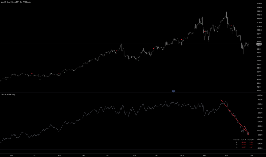
Adaptive Trend ChannelAdaptive Trend Channel is designed to find the most reliable short-term and long-term trend channels automatically, instead of forcing the user to work with one arbitrary lookback length. The script scans a broad range of candidate periods, builds a regression-based channel for each one, and then compares them through a multi-factor selection process. The goal is not just to find a channel that looks clean, but one that is statistically solid and structurally meaningful. To do that, the indicator favors channels with strong linearity, efficient trend behavior, sufficient directional strength, good price containment inside the bands, controlled width, and stable quality across nearby lengths. This helps avoid weak or accidental fits and gives priority to channels that are more robust in practice.
For best results, it is strongly recommended to use a logarithmic chart and to enable the option "Enable for logarithmic price scale" in the indicator settings. This is especially important on assets with large percentage moves over time, because the channel geometry then reflects percentage-based price movement more accurately.
Color is also important and very simple to read:
if a very robust channel is found, it is displayed in blue by default. This means the selected channel passed the eligibility filters and qualified as a strong structure. If no channel is robust enough, the script can still display the best available candidate, but it will appear in gray by default.
OVERVIEW
Adaptive Trend Channel helps identify the best short-term and long-term trend channels without manually testing many different lengths. Instead of relying on fixed settings, it adapts to the market structure by selecting the channels that best balance fit, strength, consistency, and usability.
The indicator can display:
- the best short-term channel
- the best long-term channel
- an optional midline
- an optional data table with channel diagnostics
HOW IT WORKS
For each tested lookback period, the script builds a regression-based trend channel and measures its quality.
Two selection modes are available:
1. Pearson r
This mode focuses mainly on linear fit quality.
2. Robust Composite
This mode uses a broader decision framework and combines several factors to favor channels that are not only well fitted, but also more reliable as usable trend structures.
In Robust Composite mode, the selection can include:
- Pearson correlation
- trend efficiency
- ADX trend strength
- price containment inside the channel
- channel width control
- local stability across neighboring tested lengths
A channel is considered eligible only if it passes the minimum filters defined by the user, such as:
- minimum absolute Pearson r
- minimum ADX
- minimum containment ratio
- maximum allowed channel width
If at least one eligible channel is found, the strongest one is selected and displayed in blue by default.
If none qualifies, the script still displays the best available fallback channel, but in gray by default.
WHY THIS APPROACH
A fixed-length channel can work well in one market condition and fail badly in another. This script addresses that problem by testing multiple candidate lengths and ranking them with a more complete selection logic.
The method is designed to reduce three common issues:
- choosing an arbitrary lookback period
- overvaluing channels that only look good visually
- accepting channels that fit price poorly or are too unstable
By combining fit quality, structure, strength, containment, and stability, the indicator aims to produce channels that are more trustworthy and easier to interpret.
HOW TO READ IT
- The short-term channel helps track the active market structure.
- The long-term channel helps frame the broader trend.
- Blue by default means a robust eligible channel was found.
- Gray by default means the displayed channel is the best available one, but it did not pass the eligibility filters.
- The position of price inside the channel helps show whether price is near the upper band, lower band, or midline.
FEATURES
- Automatic search for the best short-term and long-term channels
- Adaptive selection across multiple lookback lengths
- Robust eligibility filtering
- Blue default color for robust eligible channels
- Gray default color for fallback non-eligible channels
- Support for linear and logarithmic mode
- Optional midline display
- Optional table with channel metrics
- Two detection methods: Pearson r or Robust Composite
TABLE METRICS
Depending on your settings, the table can display:
- best length
- selection metric
- stability
- trend efficiency
- Pearson r
- ADX
- annualized channel return
- annualized channel price return
MAIN INPUTS
- Show Best Short-Term Channel
- Show Best Long-Term Channel
- Enable for logarithmic price scale
- Display Deviation Multiplier
- Best Channel Detection
- minimum eligibility filters for Pearson r, ADX, containment, and width
- optional table settings
NOTES
- For best interpretation, use logarithmic mode on a logarithmic chart.
- Blue by default means the channel passed the eligibility filters and was considered robust.
- Gray by default means the script is showing the best fallback channel, but it is not eligible.
- Annualized return metrics are intended for daily, weekly, and monthly timeframes.
Adaptive Trend Channel is built for traders who want a more objective, adaptive, and robust way to identify high-quality trend channels. 指标

LinReg SlopeChangeThis indicator is a precise trend-following tool that tracks the acceleration (rate of change) in the price's linear regression curve. While a standard Linear Regression (LR) indicator simply shows the direction of the price, this tool focuses on detecting whether a trend is gaining momentum or exhausting by measuring the Slope Delta.
Here is a detailed guide explaining the technical structure, parameters, and usage of the indicator:
1. Core Calculation Logic
-The indicator processes market movements through a three-stage mathematical filter:
-Linear Regression (LR): It calculates the "best-fit" line for prices over a specified period (len).
-Slope Percentage (Slope %): It calculates the difference between the current LR value and the previous bar's LR value, expressed as a percentage of the current value.
-Slope Change (Slope Delta): This is the heart of the indicator. It calculates the difference between the current slope percentage and the previous bar's slope percentage. Mathematically, this acts as the "acceleration" (second derivative) of the price action.
2. Input Parameters
-LR Length : The number of lookback bars used for the regression calculation. Higher values lag more but provide more reliable signals.
-Slope Change Threshold (%) : The minimum slope change required to trigger a signal. This can be increased to avoid false signals in noisy (sideways) markets.
-Source : The price data used for calculations (Usually set to close).
3. Signals and Visualization
The indicator operates on a sequential signal logic, meaning it does not produce consecutive "BUY" or "SELL" signals; it waits for a trend reversal.
BUY Signal: Occurs when the momentum of the slope (Slope Delta) breaks above your defined threshold_chg. It is marked by a green triangle on the chart.
SELL Signal: Occurs when the slope momentum breaks below the negative threshold. It is marked by a red inverted triangle.
Background Color: Highlights the active trend by shading the "BUY" zone green and the "SELL" zone red.
4. Usage Strategies
A. Catching Trend Reversals
Because this indicator notices weakening in the slope before the price fully turns, it can respond faster than classic Moving Averages (MA). If the slope begins to decrease (negative delta) during an uptrend, it may serve as a leading signal of a potential peak.
B. Consolidations and Breakouts
When the price is moving sideways, the slope is near zero. Thanks to the Slope Change Threshold parameter, the indicator captures the surge in momentum when price breaks out of stagnation, confirming the start of a new trend.
C. Filtering
Using this indicator in conjunction with a volume indicator (e.g., RV) or an oscillator (like RSI) will increase the success rate. It is particularly powerful for determining trend direction on higher timeframes (4H, Daily).
Note: The threshold_chg (Threshold) parameter should be adjusted according to the volatility of the pair you are trading. For volatile assets like cryptocurrencies, keeping this value slightly higher will reduce "whipsaw" or false signals. 指标
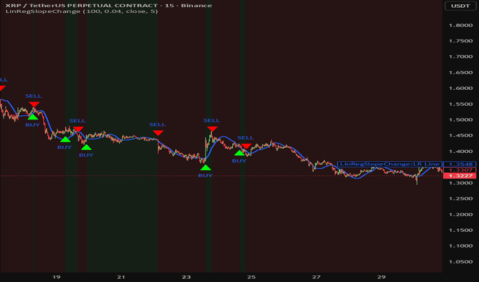
Adaptive Trend ChannelAdaptive Trend Channel is a trend-following overlay indicator designed to visualize directional bias through a dynamic centerline and a volatility-based channel.
The script does not try to predict exact tops or bottoms. Its purpose is to help the trader structure price movement into bullish and bearish phases and track where the active side of the market is currently being defended.
How it worksThe indicator is built from three core elements:
1. Linear regression smoothing
The script first applies linear regression to high, low, and close. This reduces local noise and creates a smoother representation of recent price movement.
2. Reaction envelope on the smoothed series
After regression smoothing, the script builds a short reaction structure using:
an SMA of the regressed highs and lowsa highest/lowest window over the same smoothed dataThis envelope is used to detect whether recent price behavior continues to support the current directional regime or starts to weaken.
3. ATR-based channel width
The channel width is not fixed. It is scaled using ATR, so the distance from the centerline expands and contracts with market volatility.
This allows the channel to remain relatively narrow in calmer conditions and wider during more volatile phases.
Regime logicThe script maintains a stateful market regime:
Bullish regime: the centerline trails upward using the strongest recent trough structureBearish regime: the centerline trails downward using the weakest recent peak structureA regime change happens only when the smoothed reaction structure breaks against the current direction and the regressed close confirms that shift.
This means the channel is not simply redrawn on every minor fluctuation.
Instead, it attempts to preserve directional continuity until there is enough evidence to flip.
What is displayedThe indicator plots:
a central adaptive trend linea lower active channel boundary during bullish conditionsan upper active channel boundary during bearish conditionsa colored fill showing the currently dominant sidecircular markers at regime flipsGreen indicates bullish control.
Red indicates bearish control.
How to use itThis script can be used as a market structure and trend context tool.
Typical ways to read it:
When the channel is bullish, the centerline and lower boundary can be used as a reference zone for continuation behaviorWhen the channel is bearish, the centerline and upper boundary can be used as a reference zone for rejection behaviorRegime flips can help identify transitions from one directional phase to anotherThe slope of the centerline can help assess whether the current trend is strengthening, flattening, or reversingThe tool is generally more useful for trend context than for isolated entry signals.
It can also be combined with price structure, liquidity zones, support/resistance, or volume-based confirmation.
InputsLinear regression span: controls how much smoothing is applied to the source seriesEnvelope reaction length: controls the short-term reaction window on the smoothed structureHalf-channel ATR factor: controls how wide the adaptive channel is relative to volatilitySmaller settings will make the channel react faster.
Larger settings will generally make it smoother and slower.
NotesThis indicator is intended for chart analysis and trend interpretation.
It should not be treated as a standalone trading system or as a guarantee of future market direction.
Like any trend-following tool, it may react later during sharp reversals and may produce more frequent regime changes in choppy conditions. 指标