Gold – Room for Extension or a Potential Short Term Top?At the start of August Gold traders received official confirmation that global central banks led by China’s PBOC remained buyers of Gold when prices dipped down below 4000 in mid-July. This news, coupled with a cooling of Federal Reserve rate hike expectations, helped support a technical breakout above 1 month range highs at 4166 (July 22nd high) on August 5th.
While the up move initially took a brief pause around the 4450 area to absorb a wave of profit taking, last week’s surprise intervention by the US Treasury in the bond market to stem a troublesome rise in yields had the knock-on effect of driving down the US dollar. This in turn helped make Gold, which is priced in the currency more appealing to global investors, helping push Gold prices up to 3-month highs at 4632 on Friday, before drifting off to close the week at 4605.
Looking forward, with Gold jumping 0.8% to 4642 on the Monday open, traders may be keen to hear further details of new fiscal initiatives to address soaring government borrowing costs that US Treasury Secretary Scott Bessant teased markets with at the back end of last week. They could also be preparing for the keynote speech from Fed Chair Kevin Warsh which is due to be delivered during the Fed’s Jackson Hole Symposium on Friday (1500 BST). Any further details he may reveal regarding whether policymakers could hike interest rates in mid-September may play a big role in determining if Gold prices push up to new highs or retrace back down to lower levels.
Given that the initial move above 4166 and then 4450 was supported by the technical backdrop, taking time to review the current technical update below and take stock of potential key support and resistance levels, may be helpful for setting risk and reward parameters across the next 5 trading days.
Technical Update: Could a Resistance Break Open Scope to Higher Levels?
Recovery themes have dominated activity for Gold across July and August, with the popular shiny metal staging an 18% rebound after a prolonged phase of weakness between the January 29th high at 5598 and the June 30th low of 3943. This on-going recovery could be encouraging for Gold bulls, especially as prices closed on Friday above what might have been expected to be an important resistance level.
As the chart above shows, the latest activity in Gold has seen a break above 4573, a level equal to the 38.2% Fibonacci retracement of the entire January to June decline.
Potential Resistance Focus:
The successful close above resistance at 4537 (38.2% retracement) could open the way for further attempts at price strength over upcoming sessions. Within technical analysis, closes above a 38.2% Fibonacci retracement level can shift the focus for traders to identifying higher resistance points that could now be tested.
In this scenario, traders may now be looking to the 4770/74 area, which contains the 50% retracement and May 12th high, as the next potential resistance focus. If this range is broken on a closing basis, it may open the possibility for tests of 4889 (April 17th high), and then 4966 (61.8% Fibonacci level).
Potential Support Focus:
Of course, a close above a 38.2% retracement level isn’t a guarantee of further price strength, so it remains prudent to monitor possible support levels in case sentiment turns down again. As such, 4488 (half of last week’s strength) may be viewed as the first key support. Closing breaks below this level could signal the potential for further Gold price weakness.
If 4488 were breached on a closing basis, downside risks could turn toward 4385 which is the 38.2% retracement of the rally from the June 30th low (3943) into the latest high on August 24th (4657). A closing break below 4385 might then lead to further declines, shifting focus for moves back down toward 4301 (50% level).
The material provided here has not been prepared accordance with legal requirements designed to promote the independence of investment research and as such is considered to be a marketing communication. Whilst it is not subject to any prohibition on dealing ahead of the dissemination of investment research, we will not seek to take any advantage before providing it to our clients.
Pepperstone doesn’t represent that the material provided here is accurate, current or complete, and therefore shouldn’t be relied upon as such. The information, whether from a third party or not, isn’t to be considered as a recommendation; or an offer to buy or sell; or the solicitation of an offer to buy or sell any security, financial product or instrument; or to participate in any particular trading strategy. It does not take into account readers’ financial situation or investment objectives. We advise any readers of this content to seek their own advice. Without the approval of Pepperstone, reproduction or redistribution of this information isn’t permitted.
GC GEX - Breakout Above 4690Gold futures are extending a strong daily rally, with price near 4731 after clearing the 4690 call wall. That strike was the largest call NETGEX on the map — resistance that has now flipped into the first support of the breakout.
The bid is not only technical. Last week the bond market set the cross-asset tone. The 10-year finished near 4.73% and the 30-year moved toward 5.27% , the highest area since 2007. After that selloff, the Treasury said it would at least double selected long-dated buybacks in the 10- to 30-year sector. Yields dipped, the dollar weakened, and gold and bitcoin both caught the same bid. What matters for gold is that the metal kept grinding higher even after the long end recovered most of that buyback relief . That is less a simple "yields down, gold up" tape and more a dollar-weakness / fiscal-credibility bid — the same liquidity signal that lifted crypto, expressed in bullion.
Oil and Middle East supply risk added a second inflation input. This week still has July PCE and Chair Warsh at Jackson Hole , so the rates narrative can reprice quickly. The GEX map is what frames how that reaction may travel.
🔶 Regime Context 🔶
Price is trading well above 4565 HVL , keeping GC inside a positive GEX regime . Above the gamma flip, price action typically becomes more controlled than it is below HVL. The current rally also sits above both the 50 SMA and the 200 SMA , after price retested the 200 SMA and then accelerated.
🔶 Options Structure Context 🔶
👉 4690 – C1 (highest call NETGEX wall — now cleared)
👉 4850–5000 – call cluster — next upside reference on the profile
With C1 accepted overhead, GC has entered the positive gamma extension zone . That opens gamma squeeze potential toward that call cluster, as long as acceptance holds above the old wall.
🔶 Downside Structure 🔶
👉 4690 – flipped C1 — first breakout support
👉 4565 – HVL — regime pivot
👉 3585 – P1 — strongest put wall, well below the current range
Losing 4690 would turn this from an extension into a failed breakout test. A daily move back through 4565 HVL would be the larger regime warning. The 3585 put wall is a distant floor, not nearby structure.
🔶 Options Sentiment 🔶
CALL$ 72.1% means call options at an equivalent distance from spot are priced 72.1% higher than the corresponding puts — this is elevated call pricing skew .
On the Options Oscillator, the filled green histogram remains elevated at the right edge — call pricing skew is still strong, not fading from this move.
IVRank 39.1
CALL$ 72.1% — call pricing skew
🔶 Macro Catalyst 🔶
Treasury's larger long-end buybacks, a weaker dollar, and still-elevated long yields are the fundamental stack behind this surge. PCE and Jackson Hole can reset the rates side of that story. Structure first; headlines second.
🔶 Key Structure to Watch 🔶
4690 — C1, breakout support
4850–5000 — call cluster / extension target
4565 — HVL / regime pivot
3585 — P1, distant put wall
For now, GC is holding in a positive GEX regime above HVL, with the 4690 call wall cleared and price working inside the extension zone.
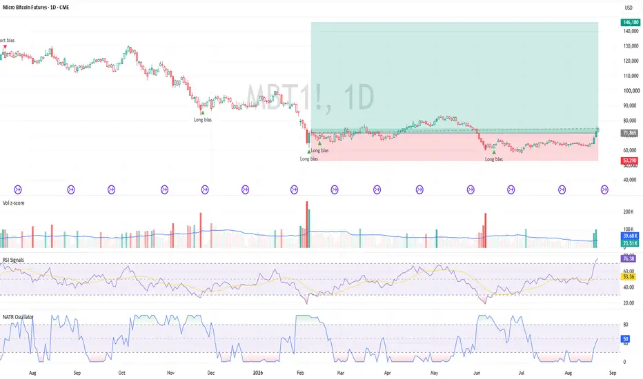
The key question is whether momentum can carry price into the 4850–5000 call cluster — and how the market reacts once it gets there. Crypto Market Overview: Multi-Leg Breakout After Prolonged RangeAfter weeks of compressed, low-volatility trading that left many assets looking lifeless, crypto markets staged one of their strongest weekly performances in recent memory. Bitcoin broke out of a multi-month range and advanced up to $79500 (Coinbase spot), with several large-cap alts posting even larger percentage gains. The move reversed months of bearish or range-bound sentiment in short order.
Primary drivers
1. Treasury / bond market signal
The U.S. Treasury's decision to at least double the size of its long-dated bond buyback operations helped pull the 30-year yield down. Lower long-end yields improved risk appetite across asset classes. While not quantitative easing, the move was widely interpreted as a supportive liquidity and signaling event for risk assets, including crypto.
On 19 August the Treasury raised the maximum size of its liquidity support buybacks for longer-dated securities from $2 billion to at least $4 billion per operation. The change is effective 9 September and runs through 4 November. The 30-year — which had hit above 5.33% on Tuesday, its highest since June 2007 — fell more than 10 basis points to 5.184% on the announcement.
That's the catalyst. A technical operation in the government bond market, not yet in effect, that moved a yield by a fraction of a percent. And it's credited with a roughly +25% week in bitcoin.
It gets stranger. The move unwound almost immediately — by Thursday the 30-year had given back the entire drop and the 10-year sat at 4.704%, above where it was before the announcement. The long bond finished the week around 5.27%, essentially back where it had been before the Treasury stepped in.
Crypto kept climbing for three more days after the trigger had already reversed. Which tells you something about where the energy was actually stored.
2. Spot ETF buying power
U.S. spot Bitcoin ETFs recorded $606.29 million in net inflows on 20 August, their largest single day since 1 May, following $517.19 million on the 19th, $189.30 million on the 18th and $297.56 million on the 17th. Four consecutive days, roughly $1.61 billion. Ethereum funds ran a parallel streak, adding $189.15 million on the 19th — their largest single day in ten months — and $221 million on the 20th.
These are actual share creations that require spot purchases and represent one of the more durable sources of demand in the current market structure.
3. Rare short-dominated liquidation event
Derivatives markets saw one of the largest overall liquidation days on record (ranked roughly 7th–8th historically by several data providers). Critically, the vast majority of the forced closures were short positions (estimates of $2.7–3B+ in a single day and over $4B across the core window). Most historic mega-liquidation events have been long liquidations during sell-offs. A short squeeze of this scale is unusual and mechanically amplified the upward move while it lasted.
4. Policy / narrative support
The White House hosted crypto executives the next day, where Trump pushed Congress to pass a fair version of the Clarity Act. Parallel regulatory signals, including SEC rulemaking proposals, added to the tone. All of it helped sentiment. But none of it moved the yield curve, and headlines like these have arrived before without producing a week like this — which is why I'd put them behind the macro and positioning factors above.
Positioning and market character
The preceding period left markets heavily short or under-positioned after a long grind. The combination of a macro catalyst and forced covering produced the classic cascade. Volume and open-interest shifts reflected the intensity of the squeeze. Sentiment indicators flipped rapidly from fear/neutral toward greed territory.
A squeeze on its own is mechanical. Forced buying creates more forced buying, and when the fuel runs out the move usually gives some back. So the more useful question is whether anything underneath it was actual demand. The ETF flows are the strongest evidence that some of it was — those require someone to go out and buy spot. Different quality of demand than a short closed at a loss.
Balanced outlook
Does the breakout have legs? Who knows — I guess we'll find out soon (as Sadie Sink put it when asked about her role in Spider-Man: Brand New Day).
The structural leg that actually held is ETF demand. The other one didn't — long-end yields reversed within a day and finished the week higher, which makes the macro support look more like a sentiment event than a change in conditions. Residual short covering or fresh speculative interest can still contribute.
At the same time, a move of this velocity almost always invites profit-taking, consolidation, or a healthy dig lower to reset leverage and shake out late entrants. Such a pullback would be normal rather than necessarily trend-ending.
Legislative developments (Clarity Act progress or lack thereof) will continue to influence narrative and risk premium, but markets have already begun pricing improved regulatory expectations. Actual passage, if it occurs, could face classic "buy the rumor, sell the news" dynamics after the anticipatory move already seen. Failure or further delay would likely reintroduce uncertainty.
What I'll be watching:
Whether ETF flows hold once price stops going up. Long-end Treasury yields, since this started there and has already partly unwound. Funding and open interest, because a squeeze clears out one side of the book and leaves room for the other. And 15 September, the Senate's first procedural vote on the Clarity Act — expectations are already partly priced, which introduces the usual risk of a sell-the-news reaction even on a good outcome.
Next week should give more clues about whether it holds.
The calendar includes events such as Core PCE (the Fed's preferred inflation gauge), the second estimate of Q2 GDP, and Jackson Hole, where Kevin Warsh delivers his first keynote as Fed chair on Friday 28 August. Watch how Bitcoin holds key levels through these events — sustained support would favor continuation of the upmove; a clean break lower would signal the need for more consolidation.
Overall, the breakout was driven more by positioning and liquidity than by any single headline. The market has shifted from a low-energy range into a more dynamic phase, with the usual crypto volatility that accompanies such transitions.
The weekend has been choppy, and the alts have shown it most — some large caps dropped double digits and recovered most of it inside a session. This piece focuses on bitcoin, but the same drivers run through the rest of the market, usually with more amplitude.
I'll be following it closely from here, and if I'm honest about my own lean it is mildly bullish. I can't make that case from the data above — the data says digest and consolidate. It's a feel, from having watched this market for a long time: crypto tends to move while everyone is still working out what happened last week. Speculation on my part, and I've been wrong before.
What's your read — is this the start of a real breakout, a trap for late buyers, or something in between? Share your thoughts in the comments.
Thank you and enjoy your trading 😊
 Long
Long
 Long
Long
Bitcoin news: BTC reclaims $74,000 as ETFs see $5.3B volumeBitcoin’s latest rally has been backed by a sharp increase in institutional activity. U.S. spot Bitcoin ETFs recorded more than $5.3 billion in trading volume as BTC reclaimed $74,000 for the first time in 86 days.
BlackRock’s IBIT dominated activity with $4.44 billion in volume. Fidelity’s FBTC came next at $438 million and Grayscale at $208.8 million. Meanwhile, Bitwise, ARK Invest, VanEck, Morgan Stanley, Franklin Templeton, Invesco, Valkyrie, WisdomTree and Hashdex accounted for the remaining volume as per data.
$517M Flows as Bitcoin Jumps 17%
U.S. spot Bitcoin ETFs also attracted $517.19 million in net inflows, their strongest inflow day since May 4. Eight of the 12 funds recorded positive flows. BlackRock’s IBIT led with $284.7 million, followed by ARK and 21Shares’ ARKB at $77.7 million. Fidelity’s FBTC came next at $62.4 million.
The ETF activity came as Bitcoin surged roughly 17% in two days. It added around $11,000 and more than $220 billion to its market capitalization.
The rally has also triggered a major short squeeze. More than $3.6 billion in short positions have been liquidated over the past 72 hours, including $2.75 billion in Bitcoin shorts on Wednesday. Over the following 24 hours, another $783.2 million in Bitcoin positions were liquidated. Of this, $747.7 million came from shorts, according to CoinGlass data.
What Fueled this Rally?
The rally followed the U.S. Treasury Department’s decision to at least double liquidity-support buyback operations for longer-dated nominal coupon securities. This applies in the 10- to 30-year segment.
Additional catalysts included the SEC’s latest crypto proposal. There was also a White House meeting between President Donald Trump and prominent crypto executives, helping trigger the unexpected move higher.
McGlone Warns Rally Could Fade
Despite the surge, Bloomberg’s Mike McGlone remains bearish. He described the move as “a bounce within the purge”, arguing that August can produce short squeezes even during a broader bear market.
McGlone criticized Bitcoin’s volatility and correlation with stocks, saying institutional investors face unfavorable risk-reward characteristics. He also argued that the rapid expansion of the wider crypto market has created excessive supply. Consequently, he expects Bitcoin to potentially roll over by year-end.
While he supports blockchain technology, McGlone argues Bitcoin’s original peer-to-peer cash use case has weakened. This comes with the emergence of crypto-dollar alternatives. Long 
 Long
Long
Sharpe Ratio Part 1: Practical Applications & Interpretation📊 Sharpe Ratio Part 1: Practical Applications & Interpretation
Stocks • Portfolios • Trading Strategies • Rolling Analysis • Sharpe vs. Sortino
Developed by Nobel laureate William F. Sharpe, the Sharpe Ratio is one of the most widely used measures of risk-adjusted performance. It can be found in strategy backtests, fund fact sheets, TradingView strategy tester summaries as well as in extensive finance literature.
1️⃣ Sharpe Ratio — The Basic Concept
The Sharpe Ratio measures how much excess return is generated for each unit of return variability.
Sharpe = (Rₚ − Rf) / σₚ
Where:
Rₚ = portfolio or strategy return
Rf = risk-free return
σₚ = standard deviation of returns
For daily data, an annualized Sharpe is commonly calculated as:
Sharpe annualized = Mean(Excess Daily Return) / STD(Excess Daily Return) × √252
📌 Key Point: A higher Sharpe generally means that returns were achieved more efficiently relative to volatility.
💡 Example
Suppose two investments have the following results:
Investment A — Return 20%, Volatility 20%
Investment B — Return 18%, Volatility 12%
Investment A has the higher return, but Investment B may have the higher Sharpe because it achieved its return with substantially lower variability.
📌 Key point: Sharpe is not a return ranking. It is a risk-adjusted return ranking.
A more concrete walk-through makes this easier to apply. Suppose a ticker’s closing price behaves as follows over six sessions:
Day 1: $100.00
Day 2: $101.50 (+1.50%)
Day 3: $99.80 (−1.67%)
Day 4: $102.30 (+2.51%)
Day 5: $101.90 (−0.39%)
Day 6: $103.40 (+1.47%)
Mean(Daily Return) ≈ 0.68%, STD(Daily Return) ≈ 1.68%
Assuming a negligible daily risk-free rate, the daily Sharpe is approximately 0.68 / 1.68 ≈ 0.41. Multiplying by √252 gives an annualized figure — note that with only five observations this is for illustration only; real calculations should use a much longer return history (typically one to several years of daily data) before the annualized number is statistically meaningful.
📈 General Interpretation for Annualized Sharpe Values
< 0 — Poor / negative risk-adjusted return
0–0.5 — Weak
0.5–1.0 — Moderate
1.0–2.0 — Good
2.0–3.0 — Very good
> 3.0 — Exceptional, often difficult to sustain
📊 Chart Description
The chart above displays 3 companies with different paths. Despite all three companies having the same 8% annualized arithmetic mean return, their different volatility produces very different price paths and compounded outcomes.
Company C (Sharpe 2.00, Vol 4%) climbs in a steady, low-noise path with the lowest volatility and ends with the highest compounded growth (CAGR 8.2%).
Company A (Sharpe 0.45, Vol 17.8%) follows the most volatile path, with large swings and spikes above +45%, and ends with the lowest terminal value (CAGR 6.6%) despite an identical average return.
Company B (Sharpe 1.0, Vol 8.0%) has a Sharpe Ratio more than double that of Company A and half that of Company C. Its path is smoother than Company A's but more volatile than Company C's, resulting in a (CAGR 8.0%).
🎯 Key Takeaway: Sharpe Ratio favors higher excess returns and lower volatility. Two investments can generate similar returns, yet the one achieving them with less volatility can have a much higher Sharpe Ratio.
---
2️⃣ Sharpe Ratio for a Portfolio of Stocks
When evaluating a portfolio, Sharpe should be calculated from the portfolio's own return series.
💼 Example portfolio
AAPL — 25% weight, +2.0% return
MSFT — 25% weight, +1.0% return
NVDA — 25% weight, +4.0% return
AMD — 25% weight, −2.0% return
Rportfolio = 0.25RAAPL + 0.25RMSFT + 0.25RNVDA + 0.25RAMD = 1.25%
Rportfolio = 0.25×(+2) + 0.25×(+1) + 0.25×(+4) + 0.25×(−2) = 1.25%
Repeat this for every period to create the portfolio return series, then calculate Sharpe from that series.
⚠️ Important:** Do not simply average the individual Sharpe Ratios of the holdings. Portfolio risk depends on both the volatility of each stock and the correlations between them. Therefore, portfolio Sharpe must be calculated from portfolio returns.
The study “Buffett’s Alpha” by Andrea Frazzini, David Kabiller, and Lasse Pedersen examined the performance of Berkshire from November 1976 through December 2011.
The study found that Berkshire Hathaway, led by Warren Buffett, achieved an exceptional long-term Sharpe ratio of about 0.76 (1976–2011), compared with 0.39 for the overall stock market over the same period.
---
3️⃣ Sharpe Ratio for Comparing Individual Stocks
Sharpe can also be used to compare individual stocks, provided every stock is evaluated using the same methodology.
AAPL — Return 18%, Volatility 22%, Sharpe 0.82
MSFT — Return 17%, Volatility 18%, Sharpe 0.94
NVDA — Return 35%, Volatility 45%, Sharpe 0.78
AMD — Return 28%, Volatility 38%, Sharpe 0.74
📌 The unadjusted return ranking is NVDA > AMD > AAPL > MSFT, while the Sharpe ranking is MSFT > AAPL > NVDA > AMD.
For a meaningful cross-sectional comparison, use the same:
• Timeframe
• Lookback period
• Return calculation
• Risk-free rate
• Annualization method
• Treatment of missing data
---
4️⃣ Sharpe Ratio for a Trading Strategy
A strategy trade log might contain returns such as +5%, −2%, +8%, −4%, and +3%. It may be tempting to calculate Sharpe directly from these trades, but that is generally not the preferred approach.
The reason is that Sharpe is fundamentally a measure of returns through time. Trades can have very different holding periods, so treating every trade as one equally spaced observation can distort the time dimension.
⚙️ Preferred approach
Equity Curve → Periodic Returns → Excess Returns → Sharpe
Start with the strategy equity curve and calculate periodic returns, for example:
Jan 1: $100,000
Jan 2: $100,500
Jan 3: $101,200
Jan 4: $99,900
Jan 5: $101,000
rₜ = (Equityₜ / Equityₜ₋₁) − 1
This properly incorporates holding periods, compounding, position sizing, cash periods, portfolio exposure, overlapping positions, and the actual path of the strategy. Sharpe would be rt STD(rt)
A trade-level statistic can still be calculated as Mean(Trade Return) / STD(Trade Return), but it should be clearly identified as a trade-level Sharpe rather than the standard time-series Sharpe Ratio.
---
5️⃣ Rolling Sharpe Ratio
A single Sharpe Ratio summarizes an entire period. Rolling Sharpe is useful when market conditions or an asset’s risk-adjusted performance change over time.
With a 252-day lookback, the calculation moves forward one observation at a time:
Day 252 → Returns 1–252
Day 253 → Returns 2–253
Day 254 → Returns 3–254
The result is therefore a time series of Sharpe Ratios rather than a single number.
For a ticker, instead of an equity curve, the raw input is simply the ticker's own daily price return series (percentage change in closing price from one session to the next). A 252-day rolling Sharpe recalculates the ratio from that same series, dropping the oldest day and adding the newest one at each step:
Window 1 (Jan 2023 – Dec 2023): 1.65
Window 2 (Feb 2023 – Jan 2024): 1.58
Window 3 (Mar 2023 – Feb 2024): 1.40
Window 4 (Apr 2023 – Mar 2024): 1.05
Window 5 (May 2023 – Apr 2024): 0.62
📉 Here the rolling Sharpe drifts from 1.65 down to 0.62 over roughly sixteen months — the ticker’s risk-adjusted performance is deteriorating even though price may still be trending higher, because volatility is rising faster than return. This is exactly the kind of shift a single, full-history Sharpe would hide.
🔄 What Does Rolling Sharpe Tell Us?
Suppose a ticker has a lifetime (multi-year) Sharpe of 1.20 calculated from its full daily price-return history. That number may look healthy, but a rolling view might show its more recent risk-adjusted performance deteriorating.
Example:
1.8 → 1.6 → 1.3 → 0.9 → 0.4 = deterioration
0.3 → 0.6 → 0.9 → 1.2 → 1.5 = improvement
📌 A static Sharpe tells us what happened over a period. Rolling Sharpe tells us how risk-adjusted performance is changing through time.
⏱️ Choosing the Rolling Lookback
30 days (~1.5 months) — Very responsive, noisy
63 days (~3 months) — Short-term
126 days (~6 months) — Intermediate
252 days (~1 year) — More stable
504 days (~2 years) — Very stable, slower
There is no universally correct lookback. Shorter windows react faster but are more statistically noisy; longer windows are more stable but slower to detect changes. For strategy monitoring, 126–252 trading days can provide a useful balance. For research, examining 63/126/252 together can be especially informative.
---
⚠️ Sharpe Does Not Measure Drawdown Directly
Sharpe uses standard deviation as its risk measure. Standard deviation penalizes both positive and negative variability. This means unusually large positive returns can increase measured risk even though those returns are desirable.
Sharpe also does not specifically measure Maximum Drawdown, drawdown duration, time spent underwater, or downside-only volatility.
---
⚖️ Sharpe vs. Sortino Ratio
The Sortino Ratio is similar to Sharpe, but it changes the definition of risk.
Sharpe = (Return − Risk-Free Rate) / Total Volatility
Sortino = (Return − Target Return) / Downside Deviation
The key difference is that Sharpe treats all volatility as risk, while Sortino focuses specifically on unfavorable volatility.
For example, a strategy with occasional very large positive returns can have higher standard deviation and therefore a lower Sharpe. Sortino does not penalize those positive returns merely because they are unusually large; it concentrates on returns below the chosen target or minimum acceptable return.
🎯 Why Sortino May Be Better for Risk
For many investment and trading applications, downside risk is more relevant than total volatility. Investors generally welcome upside surprises, while downside surprises are what threaten capital.
Return — Strategy A 20%, Strategy B 20%
Upside volatility — Strategy A High, Strategy B Low
Downside volatility — Strategy A Low, Strategy B High
Sharpe — Strategy A Similar, Strategy B Similar
Sortino — Strategy A Higher, Strategy B Lower
Sharpe may view both strategies as similarly risky because both have substantial variability. Sortino recognizes that Strategy A's variability comes primarily from positive outcomes, while Strategy B's comes primarily from negative outcomes.
Therefore, Sortino may be more intuitive and potentially more informative when the primary concern is downside risk rather than total volatility.
🤔 Sharpe or Sortino?
Neither metric is universally superior. They answer different questions:
Sharpe asks: How much excess return did I generate per unit of total volatility?
Sortino asks: How much return did I generate per unit of downside risk?
Sharpe remains highly useful when total volatility is relevant. Sortino can be more investor-relevant when the main concern is losses and unfavorable returns. For trading strategies, it is generally better not to rely on either metric alone.
---
🏁 Final Takeaway
The Sharpe Ratio is powerful, but its value depends on using the correct return series.
📌 For individual stocks: calculate Sharpe from the stock's periodic returns.
📌 When comparing different assets across different timeframes: it is critical to ensure the Sharpe Ratios use consistent return definitions, risk-free rates, lookback periods, and annualization methods.
📌 For portfolios: calculate it from portfolio returns—not from the average Sharpe of its holdings.
📌 For strategies: preferably calculate it from the equity curve's periodic returns rather than treating individual trades as equally spaced observations.
📌 For monitoring: use a rolling lookback such as 63, 126, or 252 periods to see whether risk-adjusted performance is improving or deteriorating.
📌 When the primary concern is downside risk rather than total volatility: Sortino may provide a more investor-relevant perspective.
Ultimately, no single ratio describes the whole picture. Sharpe measures return relative to total volatility; Sortino measures return relative to downside risk; and Martin Ratio measures return relative to drawdown-related risk. Used together, they provide a more complete picture of risk-adjusted performance.
📝 Note
Sharpe ratio applications are extensive, interested users should explore more applications and methodologies.
📚 Sharpe Ratio Part 2: 5 Common Calculation Errors
Explains how to avoid the most common mistakes when calculating and interpreting the Sharpe Ratio—from inconsistent return periods and incorrect annualization to invalid volatility calculations and other methodological pitfalls.
Sharpe Ratio — Educational TrendAdvantage Reference  Education
Biggest Short Liquidation Ever: Is This a BTC Reversal?⏱️ Reading time: 3 minutes
🔹 Biggest Short Liquidation Ever
The recent move is especially striking because the liquidation spike came from the short side. According to data cited in current market reports, roughly $2.7 billion of crypto short positions were liquidated over 24 hours, the largest wave of forced short closures in records going back to 2021.
That makes the event historically important. But does it make Bitcoin’s reversal confirmed?
⛽ Liquidations are fuel, not a signal
A short liquidation happens when a leveraged bearish position is forcibly closed as price rises. The exchange effectively has to buy back the position, creating additional demand.
This creates a feedback loop:
Price rises → shorts approach liquidation → forced buying begins → price rises further → more shorts are liquidated.
That mechanism can turn an ordinary rally into a vertical squeeze.
🔥 Why the current liquidation matters
The latest liquidation spike stands out against much of the historical series, showing that this was not simply another routine derivatives flush. But the important distinction is between historical magnitude and directional confirmation.
A record liquidation event tells us that positioning was unusually vulnerable. It does not tell us that Bitcoin has automatically entered a new bullish trend.
This distinction is easy to miss because the price and liquidation charts move together during a squeeze. The liquidation itself helps explain why the move became so powerful, but it is not necessarily the original reason buyers appeared.
That is why large liquidations are better understood as a measure of leverage being removed from the market than as a standalone reversal indicator. Unusually large liquidation waves can amplify price movement, but their occurrence alone does not establish a trend change.
🚀 What would make the reversal more convincing?
This is where the price structure becomes more useful than the liquidation headline.
On the daily chart, Bitcoin has moved back into an overhead zone around $73,000–$74,000 , followed by another resistance area around $77,000–$78,000 .
That creates a simple setup:
1) Liquidations show positioning stress.
2) Price structure shows whether that stress produced a lasting breakout.
3) Open interest shows whether leverage is being rebuilt.
4) Spot demand helps determine whether the move has support beyond forced derivatives buying.
The most interesting scenario would be one where Bitcoin holds above the reclaimed resistance area while the market continues to attract genuine spot demand. In that case, the short squeeze may have acted as the ignition mechanism for a broader recovery.
The alternative is less dramatic: shorts get cleared, price reaches overhead supply, and the market returns to its previous range.
That is why the reaction after the squeeze can be more informative than the liquidation spike itself.
If this post was useful, feel free to boost 🚀 it and share your view in the comments 💬
⚠️ Disclaimer: This publication is for educational and informational purposes only. It does not constitute financial, investment or trading advice. Market conditions can change, and readers should do their own research and manage risk accordingly.
Education 
Germany 40 – Facing a Potential August Sentiment CrisisThe strength and longevity of the recent surge to new all-time highs at 26595 (August 12th) in the Germany 40 has been called into question this week as bullish sentiment toward the index has been hit hard by a spike in global bond yields which has reflected growing concerns amongst traders regarding inflation risks at a time when the situation between the US and Iran in the Middle East seems to be deteriorating again.
Throw in worries about the increased borrowing by several key companies to fund their artificial intelligence build outs alongside a fresh wobble in demand for chipmaker stocks, and it’s perhaps easier to understand why after opening on Monday at 26495, the Germany 40 has dropped down to test some potentially important technical levels around the 26000 level at the time of writing (0645 BST). More on this in the technical update below.
Looking forward, while traders may be keeping a close watch on events in Iran and the direction of global bond yields, which eased back from their recent highs yesterday, sentiment toward the Germany 40 index into the weekly close could also be impacted by the release of the latest preliminary PMI surveys on Friday for Germany at 0815 BST and the Eurozone at 0900 BST. Readings above 50 signify economic expansion, while below 50 suggest economic contraction. Any indication from these surveys that economic growth may be starting to stall again moving through Q3 could weigh on index prices, while stronger data could be taken more positively.
Technical Update: Failure at Resistance But Watching Support:
So far this week the Germany 40 index has seen selling pressure develop to reverse recent price strength and prompt a setback. Interestingly, from a technical perspective, as the chart below shows, this setback has materialised after consistent failure to close above what may be viewed as a key resistance at 26451. This level is equal to the 38.2% Fibonacci extension of the sell‑off seen between 25942 (July 6th high) and 24617 (July 17th low).
Moving forward into early next week, traders could now be wondering whether the current price weakness may develop into a more extended phase of declines or could simply be a limited correction within an ongoing uptrend. At such a pivotal time, identifying potentially important support and resistance levels that may prove instrumental in determining the next directional themes for the Germany 40 index, may be an invaluable aid to decision making.
Potential Resistance Levels:
As suggested above, the 38.2% Fibonacci extension level at 26451 could represent the first key resistance, especially given it capped prices and helped to establish this week’s latest declines. As such, closing breaks above 26451 may now be required to open the way for challenges of higher resistance points.
A close above 26451 could shift attention toward the next resistance level at 26763 (61.8% extension). A break above 26763 could then open the way for moves toward 27269 (100% extension).
Possible Support Levels:
While resistance at 26451 continues to cap Germany 40 prices on a closing basis, it could leave open the possibility of slowing upside momentum. If this is the case, the first support may be 26037, which is the current level of the Bollinger mid‑average.
As the chart highlights, closing breaks below 26037 could shift focus toward the next potential support at 25846 (38.2% Fibonacci retracement). Closes below 25846, if seen, could then open the way for declines to 25613 (50% retracement), and even 25380 (61.8% level).
The material provided here has not been prepared accordance with legal requirements designed to promote the independence of investment research and as such is considered to be a marketing communication. Whilst it is not subject to any prohibition on dealing ahead of the dissemination of investment research, we will not seek to take any advantage before providing it to our clients.
Pepperstone doesn’t represent that the material provided here is accurate, current or complete, and therefore shouldn’t be relied upon as such. The information, whether from a third party or not, isn’t to be considered as a recommendation; or an offer to buy or sell; or the solicitation of an offer to buy or sell any security, financial product or instrument; or to participate in any particular trading strategy. It does not take into account readers’ financial situation or investment objectives. We advise any readers of this content to seek their own advice. Without the approval of Pepperstone, reproduction or redistribution of this information isn’t permitted. BTC Daily Breakout, Bullish FVG & Potential Retest GM BTC Daily Breakout, Bullish FVG & Potential Retest
After today’s strong bullish displacement, BTC has broken above the previous Daily structure, giving us a Daily BOS .
If the Daily candle closes around the current level or higher,
I’ll be watching this newly created Daily Bullish FVG as a potential area for a future retracement.
I’m not interested in chasing a +6% move.
My preferred scenario would be:
Daily BOS → Bullish Displacement → Retracement into the Daily FVG → LTF Confirmation → Potential Continuation Higher
If price retraces into the FVG, I’ll move down to the lower timeframes and wait for my system to provide a valid bullish trigger.
Above price, the Daily Equilibrium around 70K is the first area I’m watching.
If bullish momentum continues through that area, my next major HTF point of interest sits around 73–74K, where the Daily Bearish Order Block is located.
This does NOT mean BTC has to follow the path drawn on my chart.
The drawing simply represents one possible scenario out of many.
If price reaches my area but there is no lower-timeframe confirmation, there is no reason for me to enter.
If price continues higher without giving me the retracement, I won’t chase it either.
No system trigger = No trade.
My job is not to predict where every candle will go.
Identify the structure.
Mark the POI.
Wait for the market.
React when the system confirms.
These are only my personal market thoughts and trading journal.
Not financial advice and not educational content.
I’m simply sharing my journey as I learn, improve, and work toward managing my own portfolio for a living. Long 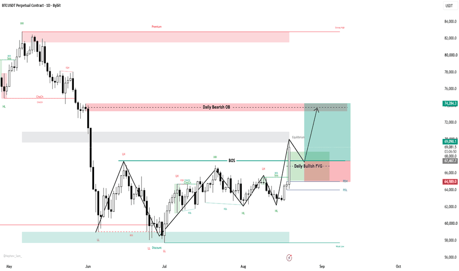
Short 
VIX - Hedge or Spec?Looking at TVC:VIX this week, the opening print of $14.98 struck me as a little odd. You don't have to stick your head out far to see there's more than a fair share of uncertainty around the globe this summer, and for market-oriented folk I am sure by now you are feeling the heat.
The omnipresent blip on every trader's radar, the conflict in Iran, and tenuous logistics surrounding the strait of Hormuz persists. Yet I can scarcely imagine a professional who is jumping into Crude Oil NYMEX:CL1! crude longs at the rumor, or even the outright news of a flare up by now. The heavy hitters called this one baked in back in April, and the print has read true on this verdict since. We still see elevated prices compared to the better part of the last decade, but crude oil is not the focus of this post.
Let's take a look into some of the fallout from this price shock, and how 'priced in' may have translated into the lowest volatility print since January.
The above chart is a 1 year line chart of volatility indicators for the major market indices, S&P500 vol - TVC:VIX (blue), Nasdaq vol - CBOE:VXN (red), Dow Jones Industrial Average vol - CBOE:VXD (green), and US Bond market vol - TVC:MOVE (orange). We have laid these out on a percentage change basis, where some interesting trends emerge. We see that the three equity benchmarks are retracing to pre-conflict lows, though Nasdaq vol remains elevated we will get into that later. The benchmark for bond volatility has been trending upwards, spiked with the war but has not retraced below the lows it made in April as the market rebounded. This is important, as options contracts take a bearing of both equity and bond volatility when it comes to pricing. So we may see both VIX and MOVE as independent but correlated underlying parameters of SPX equity options, which is a growing market at this time as investors seek cheap leverage and hedging. Which begs the titular question - are we seeing speculative buying of SPX or upside hedging of the VIX?
Here we have a 5 year bar chart of VIX volatility - CBOE:VVIX (white) and VIX - TVC:VIX (pink), as well as some basic trendlines (green). For those not well versed in options pricing or fractality, implied volatility is a bit of a mathematical perplexity, but as a result we have the volatility of the volatility as a parameter that can be measured. What we clearly see is an uptrend in this measure, meaning VIX hedging is getting more expensive. This is doubly-so, if we consider that MOVE is also a parameter at play, and the uptrend there pushed options premiums higher across the board. Interestingly, where the VVIX held it's uptrend the VIX appears to break down, though neither market is producing higher highs at this time, only the VIX is threatening lower lows.
Now here is an interesting trend, that I wish to make note of, though I caution looking too deeply into. Above is a 5-year bar chart of DJIA vol - CBOE:VXD (white), above its Average True Range - ATR (lower window). The distinct pattern of this market appears to have disappeared, the range of its movements becoming suddenly very tight and orderly in late April '26, further indicated by the ATR. What this means, I cannot speculate. But investors should consider that volatility markets are under the bright lights of large institutions at this time.
Above is a messy chart, with the US 10-year benchmark yield - TVC:US10Y (white) and a handful of tech companies that have been leading the recent rally. Goldman Sachs Group - NYSE:GS (pink) is also tucked in there. These companies have been expanding rapidly, and putting a lot of debt on the table as a result. Many of us are aware of the credit implications of the 'AI boom' - which I believe under no circumstances at this time is a bubble - let me be clear. Yet as interest rates and inflation rise due to geopolitical instability, the current valuations of these markets even as they back off all-time-highs, should be considered in the light of the VIX making new lows.
Consider the long-term view, and the complexity of potential positioning on Wall Street at this time. The credit instruments involved, and the hedging flows pass through a deep market of complex derivatives, all of which see MOVE on the rise. With VVIX moving in lockstep, I would suggest that VIX is being heavily hedged against the upside, with volume across the tech sector in downtrend and the credit cycle tightening. We could see a pause at this level or further decline in equities. GOOGL GEX - Relative Strength at HVLWhile the broader tape is selling off today, GOOGL is showing clear relative strength — barely red, and sitting right on the 342.5 HVL.
Spot is 342.83, only a few ticks above the regime pivot. That is not a wide cushion. GOOGL is pinning the flip while the rest of the market is being offered.
🔶 Regime Context 🔶
Price is holding 342.5 HVL on a down tape. Remaining above HVL keeps GOOGL inside a positive GEX regime, but this is a test of the flip, not an established hold well above it. Between 340 put wall and 350 call wall, net GEX is mixed and direction can shift quickly.
🔶 Options Structure Context 🔶
👉 350 – C1 (highest call NETGEX wall)
Confluence at 350 (cumulative, 09/18, 31 DTE):
C1 — highest call NETGEX
Ab1 — largest absolute gamma
AbOI — highest absolute open interest
That makes 350 a clear reaction zone — not just a round number. A call cluster then stretches through 352.5 (C3) and 360 (C2) toward 370 . The 50 SMA is overhead near 352.5, lining up with C3.
Strongest near-term call flow is on 08/19 (1 DTE) at 345 , with 08/21 (3 DTE) also at 345 — just above HVL. Cumulative call volume (CV / nCV) sits at 345 as well. The 09/18 single-expiry call volume peak is at 350 , the same strike as C1.
If 350 is cleared and accepted, price enters the positive gamma extension zone — gamma squeeze potential toward 360 and the 350–370 call cluster.
🔶 Downside Structure 🔶
👉 342.5 – HVL — regime pivot; must hold for the relative-strength thesis
👉 340 – P1 — strongest put wall
👉 330 – P2
Confluence at 330 (cumulative, 09/18, 31 DTE):
P2 — second put wall
nPV / PV — strongest put volume
Together, this frames a put cluster from 340 down to 325 (P1, P3 at 337.5, P2, then 325). The 200 SMA sits near that lower edge. If 340 is broken, price enters the negative gamma extension zone — downside gamma squeeze risk toward 330 and the 325 cluster floor.
🔶 Options Sentiment 🔶
CALL$ 40.7% (59 DTE) means call options at an equivalent distance from spot are priced 40.7% higher than the corresponding puts — this is call pricing skew .
On the Options Oscillator, the green histogram is flattening at the right edge — call pricing skew is stable-to-fading , not building.
IVRank 12.1
IVx 29.6 (59 DTE)
CALL$ 40.7% (59 DTE) — call pricing skew
Implied move ±2.7% (±3.3)
🔶 Key Structure to Watch 🔶
342.5 (HVL) — relative-strength hold / regime pivot
340 (P1) — put wall; break opens the 340–325 cluster
350 (C1 + Ab1 + AbOI) — first real ceiling
352.5–370 — call cluster / 50 SMA overhead near 352.5
330–325 — P2 + put-flow floor
For now, GOOGL is the relative-strength name at HVL while the tape sells off.
The key question is whether 342.5 can hold and open a push into 350 — or whether a loss of 340 drags price into the 340–325 put cluster.  Short
Short
BIDU GEX - Positioning Before EarningsBIDU reports earnings tomorrow before the open, and the August 21 expiration (4 DTE) is the options window covering that print.
Price is trading near 102.5, just below HVL at 103, which keeps BIDU in a more reactive GEX regime. That places spot at the top of a wide put cluster — P2 at 101 and P3 at 100 — with the main call wall still overhead at 110.
What stands out is the split between pricing and flow. CALL$ is 84.1%, so calls are priced much richer than puts. Despite that, put volume below HVL is running well ahead of call volume on today's session. The strongest put flow on the August 21 expiration (4 DTE) is at 91, while the strongest call flow on that same expiry sits at 103 — right on HVL.
🔶 Earnings / Positioning 🔶
A heavy put cluster sitting just below HVL into an event often reflects speculative positioning around earnings — not just a static support level. That is the current 08/21 picture: puts are being worked underneath the regime pivot even as call pricing skew stays elevated.
The implied move is ±6.44% (±6.6), which maps roughly from the mid-90s toward the 109–110 call structure.
🔶 Regime Context 🔶
Below HVL at 103, BIDU shifts into a more reactive GEX regime, where price movements can become less stable. Spot is only about half a point below that pivot, so the first test is whether 103 is reclaimed — or whether the 100–101 put cluster has to absorb the move. Price also remains below the 50 SMA and 200 SMA, which sit overhead near the 108–110 call area.
🔶 Options Structure Context 🔶
👉 110 – C1 (highest call NETGEX wall)
Confluence at 110:
C1 — highest call NETGEX
nCV — strongest net call volume today
That makes 110 the main upside reaction zone on this expiry.
👉 109 – C3 + D+ — next call wall, strongest positive delta exposure
👉 115 – C2 — extension reference if 110 is cleared
If 110 is accepted, price would enter the positive gamma extension zone — gamma squeeze potential toward 115.
🔶 Downside Structure 🔶
👉 101 – P2 / 100 – P3 — put cluster just below spot and HVL
👉 91 – P1 + Ab1 + POI + AbOI + nPOI + nPV + PV
Confluence at 91:
P1 — strongest put wall
Ab1 — largest absolute gamma
POI — highest put open interest
AbOI — highest absolute open interest
nPOI — net put OI peak
nPV / PV — strongest put volume today
Together, this points to protective / speculative put positioning at 91 — the heaviest inventory and flow cluster on the 08/21 expiry.
If 91 is broken with acceptance, price would enter the negative gamma extension zone — downside gamma squeeze risk below that floor.
🔶 Options Sentiment 🔶
CALL$ 84.1% (60 DTE) means call options at an equivalent distance from spot are priced 84.1% higher than the corresponding puts — this is call pricing skew .
IVRank 49.9
IVx 50 (60 DTE)
CALL$ 84.1% (60 DTE) — call pricing skew
Implied move ±6.44% (±6.6)
🔶 Key Structure to Watch 🔶
103 — HVL / regime pivot (strongest call volume today)
100–101 — P3 / P2 put cluster
110 — C1 call wall
91 — P1 multi-confluence / strongest put flow (08/21, 4 DTE)
For now, the focus is how BIDU is positioned into tomorrow's BMO print: expensive calls, but put volume dominating below HVL on the 08/21 expiry.
The key question is whether the 100–101 put cluster and 103 HVL hold through the event — or whether the move stretches toward 110 on the upside or 91 on the downside.